2  Using SNF in practice

We now move from four patients to a larger simulated dataset. We have 60 patients measured with RNA expression and DNA methylation. Each dataset contains 60 variables.

There are three underlying patient groups. RNA separates the first group clearly, but the other two overlap. Methylation shows a different pattern: the third group is clear, while the first two overlap.

2.1 Structure in the two datasets

The plots below show the first two principal components so that the simulated structure is visible. SNF uses all 60 standardized variables in each dataset.

Figure 2.1: RNA and methylation PCA plots for 60 simulated patients. RNA isolates subtype 1, while methylation isolates subtype 3.

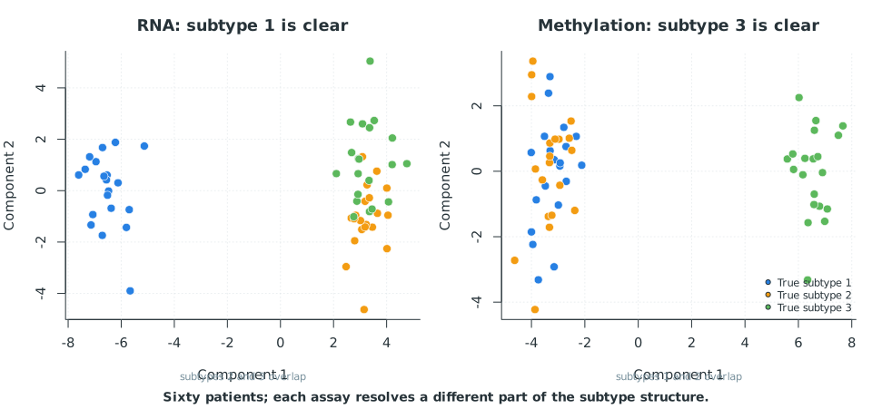
RNA and methylation therefore provide different parts of the same grouping structure.

Important

The subtype colours are shown because the true groups are known in this simulation. They are not supplied to SNF. Fusion and clustering use only the two feature matrices.

2.2 Load the data

The simulated matrices are included with the tutorial, so the R and Python code uses the same values. Patients are in rows and variables are in columns.

R

rna <- read.csv("data/simulated-rna.csv", row.names = 1,
                check.names = FALSE)
meth <- read.csv("data/simulated-methylation.csv", row.names = 1,
                 check.names = FALSE)
patients <- read.csv("data/simulated-patients.csv")

stopifnot(identical(rownames(rna), rownames(meth)))
stopifnot(identical(rownames(rna), patients$Patient))
dim(rna)   # 60 patients x 60 RNA features
dim(meth)  # 60 patients x 60 methylation features

Python

import pandas as pd

rna = pd.read_csv("data/simulated-rna.csv", index_col=0)
meth = pd.read_csv("data/simulated-methylation.csv", index_col=0)
patients = pd.read_csv("data/simulated-patients.csv")

assert rna.index.equals(meth.index)
assert rna.index.tolist() == patients["Patient"].tolist()
print(rna.shape)   # (60, 60)
print(meth.shape)  # (60, 60)

2.3 Preprocess each modality separately

SNF starts from distances, so the scale of each variable matters. A variable with a large numerical range can dominate the distance calculation even when it is not biologically more important. Here, we standardize the variables separately within RNA and methylation.

For measured data, preprocessing should be appropriate for each assay. RNA counts, methylation measurements and protein abundances usually require different transformations and quality-control steps before patient distances are calculated. Batch effects should also be investigated before fusion. SNF cannot distinguish an unwanted technical pattern from a biological one.

Here, we use Euclidean distance, K = 10 neighbours and a kernel scale of 0.5. The R code uses SNFtool (install.packages("SNFtool")), and the Python code uses snfpy.

ImportantInstalling snfpy

snfpy 0.2.2 uses interfaces from older versions of NumPy, SciPy and scikit-learn. With recent versions, it may fail with TypeError: check_array() got an unexpected keyword argument 'force_all_finite'. A compatible environment can be installed with pip install "snfpy==0.2.2" "numpy<2" "scipy<1.13" "scikit-learn<1.8". Pinning these versions also makes the Python exercises reproducible.

R

library(SNFtool)

K <- 10
sigma <- 0.5

rna_z <- standardNormalization(as.matrix(rna))
meth_z <- standardNormalization(as.matrix(meth))

# dist2() returns squared Euclidean distance, so take the square root.
D_rna <- sqrt(dist2(rna_z, rna_z))
D_meth <- sqrt(dist2(meth_z, meth_z))

W_rna <- affinityMatrix(D_rna, K = K, sigma = sigma)
W_meth <- affinityMatrix(D_meth, K = K, sigma = sigma)

Python

from snf import compute

K = 10
mu = 0.5

affinities = compute.make_affinity(
    rna.to_numpy(),
    meth.to_numpy(),
    metric="euclidean",
    K=K,
    mu=mu,
    normalize=True,
)
W_rna, W_meth = affinities

The R code uses three explicit steps to convert a data matrix to an affinity network. It standardizes the data with standardNormalization, calculates distances with dist2 and then converts the distances to affinities with affinityMatrix. Because dist2 returns squared distances, we take the square root before constructing the affinity matrix. In Python, make_affinity() performs these steps in one call for each modality.

ImportantStandardize once

By default, make_affinity() uses normalize=True and standardizes each feature column before calculating distances. This is the same z-scoring performed by the explicit standardNormalization() call in R. If the data have already been standardized, use normalize=False to avoid applying the same step twice. For these simulated data, standardization inside make_affinity() is sufficient. With measured data, modality-specific processing still comes first. RNA-seq data require appropriate transformation and filtering, while methylation data require appropriate quality control. The normalize argument handles feature scaling, not assay-specific preprocessing.

Euclidean distance is not the only option. make_affinity() accepts any distance metric supported by scipy.spatial.distance.pdist, and a different metric can be supplied for each modality as a list. For example, metric=["euclidean", "euclidean"] is equivalent to a single string here. We use Euclidean distance throughout the chapter because its geometry is easy to follow. Another metric can be used when it is more appropriate for a particular assay. The package documentation explains how a list of metrics is matched to the modalities.

At this point we have two 60-by-60 initial similarity networks. They reveal different block patterns.

2.4 Fuse the two networks

We now run 20 rounds of exchange. This is the same process used in the four-patient example. The argument t gives the number of rounds, and both packages perform the iterations internally.

R

T <- 20
W_fused <- SNF(list(W_rna, W_meth), K = K, t = T)
dim(W_fused)

Python

t = 20
fused = compute.snf(*affinities, K=K, t=t)
fused.shape

Both workflows carry out the same two stages. First, make_affinity() in Python, or standardNormalization() followed by dist2() and affinityMatrix() in R, converts each sample × feature matrix to a sample × sample affinity network.

RNA:          60 patients x 60 genes  ->  60 x 60 RNA affinity network
Methylation:  60 patients x 60 CpGs   ->  60 x 60 methylation affinity network

Second, SNF() or compute.snf() takes the two affinity networks and performs the iterative exchange described in the previous chapter. Each network keeps its own trusted local neighbours and uses the current values from the other network. Both networks are updated together in each round. The result, called W_fused in R and fused in Python, is one 60 × 60 patient-similarity matrix.

NoteDifferences between SNFtool and snfpy

Both workflows were run in clean environments using the same 60-patient dataset, K = 10, a kernel scale of 0.5 and t = 20. The RNA and methylation affinity matrices agreed to floating-point precision, with a maximum difference of about \(10^{-16}\). The fused matrices were not identical. snfpy does not force every diagonal entry to exactly 0.5 during its internal normalization, whereas SNFtool does. As a result, some entries in the fused matrices differ by as much as 0.09. The two matrices are nevertheless strongly correlated across patient pairs, with r ≈ 0.93. The downstream clusterings are even more similar. Spectral clustering of the two fused matrices gives nearly the same three-group partition, with an adjusted Rand index of about 0.95 between the R and Python assignments. Both also recover the simulated subtypes well, with ARI ≈ 0.90 for R and ≈ 0.95 for Python, as shown below.

Another Python implementation, snf2, provides a more compact API (pip install snf2, followed by from snf2 import make_affinity, fuse).

2.5 The fused similarity matrix

Before clustering, we examine the similarity matrices themselves. The patients are ordered by their known simulated groups so that the block structure is easy to see. These labels were not given to SNF.

Figure 2.2: RNA, methylation, and fused similarity heatmaps. The fused network has a clearer three-block structure than either individual network.

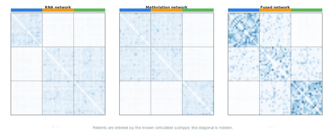
RNA and methylation each contain one boundary that is difficult to see. The three blocks are clearer in the fused network because both datasets contribute to the patient relationships.

2.6 Choosing the number of clusters

Before choosing the number of clusters, both packages provide a suggestion based on the eigenvalues of the fused network. This uses the same eigengap principle as spectral clustering.

R

estimateNumberOfClustersGivenGraph(W_fused, 2:6)

$`Eigen-gap best`
[1] 2

$`Eigen-gap 2nd best`
[1] 3

Python

first, second = compute.get_n_clusters(fused)
first, second

(2, 3)

Both methods rank 2 as the best split and 3 as the second-best. The simulation contains three subtypes, but groups 2 and 3 are closer to each other than either is to group 1. This is also visible in the weaker boundary between their blocks in the heatmap. The cluster count should therefore be assessed using biological information and stability, rather than the largest eigengap alone.

For the rest of the analysis, we use the three subtypes present in the simulation.

2.7 Spectral clustering of the fused network

R

C <- 3
cluster_snf <- spectralClustering(W_fused, K = C, type = 3)

# The labels 1, 2, 3 are arbitrary names.
table(Inferred = cluster_snf,
      Truth = patients$TrueSubtype)

        Truth
Inferred  1  2  3
       1  0  1 19
       2 20  0  0
       3  0 19  1

Python

from sklearn.cluster import SpectralClustering

C = 3
clustering = SpectralClustering(
    n_clusters=C,
    affinity="precomputed",
    random_state=1,
)
clusters = clustering.fit_predict(fused)

results = pd.DataFrame({"sample": rna.index, "cluster": clusters})
print(pd.crosstab(clusters,
                  patients["TrueSubtype"],
                  rownames=["Inferred"],
                  colnames=["Truth"]))

Truth      1   2   3
Inferred
0         20   0   0
1          0   0  19
2          0  20   1

In Python, affinity="precomputed" tells SpectralClustering that fused is already a similarity matrix rather than a table of feature vectors. Its rows should not be treated as ordinary features.

Each inferred cluster corresponds closely to one true subtype, with only one or two exceptions among the 60 patients. Cluster numbers have no intrinsic order. “Cluster 1” in one run may correspond to “cluster 3” in another, or to cluster 0 in Python. Evaluation must therefore be invariant to permutations of the labels. The adjusted Rand index (ARI) has this property. A value of 1 indicates perfect agreement, while values near 0 indicate approximately chance-level agreement.

Figure 2.3: A fused spectral embedding separates the three simulated subtypes, and an ARI bar plot compares RNA-only, methylation-only, and fused clustering.

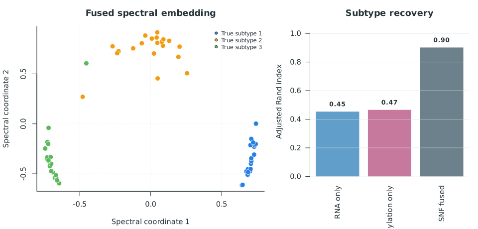
Network	ARI
RNA only	0.45
Methylation only	0.47
SNF fused	0.90

2.8 Parameters to check

2.8.1 Number of neighbors, K

K controls the size of the trusted neighbourhood. This is the same K used to construct the local matrix \(S\) in the mathematics chapter. If K is too small, such as K = 2 for 60 patients, a single noisy neighbour can dominate a patient’s row. If it is too large, the neighbourhood is no longer local because many patients are included. For this 60-patient dataset, K = 10 provides a reasonable middle ground. In the four-patient example, we used K = 2 because only four patients were available.

2.8.2 Kernel scale

The kernel-scale parameter controls how quickly similarity decreases as patients move farther apart. It is called sigma in SNFtool::affinityMatrix() and mu in snfpy::make_affinity(), and both default to 0.5. A larger value gives more weight to distant patients. A smaller value produces a sharper network that can be more sensitive to noise. Package documentation should be checked because similarly named parameters may not be implemented in exactly the same way.

2.8.3 Distance metric

Both packages compute a distance matrix before converting distances to affinities. SNFtool::dist2() calculates squared Euclidean distance. The metric argument of snfpy::make_affinity() accepts any metric supported by scipy.spatial.distance.pdist, including Euclidean and correlation-based distances. Euclidean distance is used throughout this chapter because its geometry is easy to follow. A different metric may be more appropriate for a particular assay. The package documentation should be checked because metric names and implementations can differ across packages.

2.8.4 Number of iterations

Both SNFtool::SNF() and snfpy::compute.snf() use t = 20 rounds by default, and we use 20 rounds for both implementations. It is useful to compare the results at 10, 20 and 30 rounds. Large changes across these values indicate that the resulting clusters are sensitive to the number of iterations.

2.8.5 Number of clusters

The number of subtypes should not be chosen from the appearance of the heatmap alone. The first result from estimateNumberOfClustersGivenGraph() or get_n_clusters() is also not definitive. Here, both methods ranked 2 first even though the simulation contains 3 groups. Graph-based diagnostics such as the eigengap and silhouette should be considered together with resampling stability, clinical relevance, cluster size and, where possible, external validation.

2.9 A practical workflow

In practice, first confirm that the same patients are present and appear in the same order in every dataset. Each assay should then be normalized and quality controlled according to its own requirements before distances are calculated. The individual similarity networks should be inspected before fusion because a dataset dominated by batch or another technical effect can pass that structure to the fused network.

After fusion, repeat the analysis over a reasonable range of K, kernel scales and iteration counts. The patient structure should be reasonably stable across these settings. The number of clusters is a separate downstream choice and should also be assessed for stability and biological relevance.

ImportantSNF does not repair confounding

If a sequencing batch matches a clinical group, the resulting technical split can form a strong neighbourhood and may be reinforced across modalities. Fusion combines similarity evidence. It does not determine whether that evidence is biological.

The next chapter returns to the four-patient example and works through the matrices and update rule step by step.