1  Introduction

Suppose we have four patients: A, B, C and D. We measure RNA expression and DNA methylation in each patient.

In the RNA data, A and B are close to each other. C and D are also close. The methylation data gives a different picture: B and C are the pair that stand out.

Figure 1.1: The same four patients shown in RNA and methylation space. RNA makes A-B and C-D look similar, while methylation makes B-C look similar.

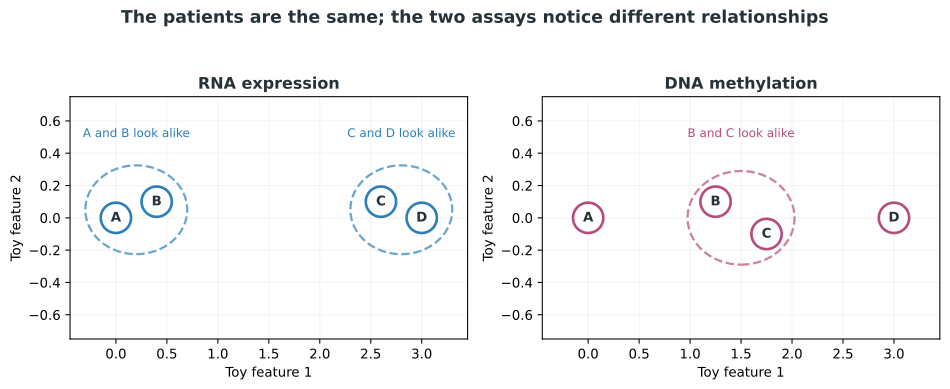
This situation is common in multi-omics studies. Different assays can reflect different biological processes and therefore show different relationships among the same patients.

The practical question is how to combine these views without forcing genes and CpG sites into the same feature table.

1.1 Constructing patient relationships

SNF changes what we compare. Instead of comparing RNA features with methylation features, we compare patients with patients within each dataset.

If two patients are close in RNA space, we draw a strong connection between them in the RNA network. If they are far apart, the connection is weak. We do the same thing for methylation.

Figure 1.2: The RNA and methylation measurements are represented as patient-similarity networks.

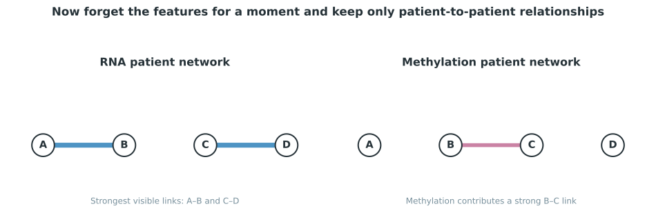
The two datasets are now represented in the same way. RNA may contain thousands of genes and methylation may contain hundreds of thousands of CpG sites, but both have been converted to patient-to-patient relationships.

At this point, the RNA view says “A goes with B” and “C goes with D”. Methylation adds another piece of information: B is close to C.

1.2 Updating RNA with methylation

Consider the relationship between A and C.

RNA initially shows little connection between A and C, but it shows a strong connection between A and B. Methylation, meanwhile, shows that B and C are strongly related.

So when RNA listens to methylation, the B-C relationship matters for A as well because B is one of A’s closest RNA neighbours.

Figure 1.3: One information exchange from methylation into RNA. RNA starts from A-B and C-D, methylation supplies B-C, and the RNA A-C relationship becomes stronger after the update.

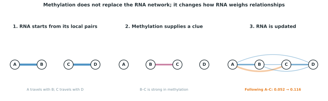
In the last panel, the RNA A-C connection changes from about 0.052 to 0.116 after one update.

The same step can be viewed in terms of local groups. RNA keeps the local pairs it already trusts, while methylation contributes a bridge between the two groups.

Figure 1.4: RNA keeps the local pairs it trusts, while methylation contributes a strong B-C bridge. That bridge gives RNA more support for A-C.

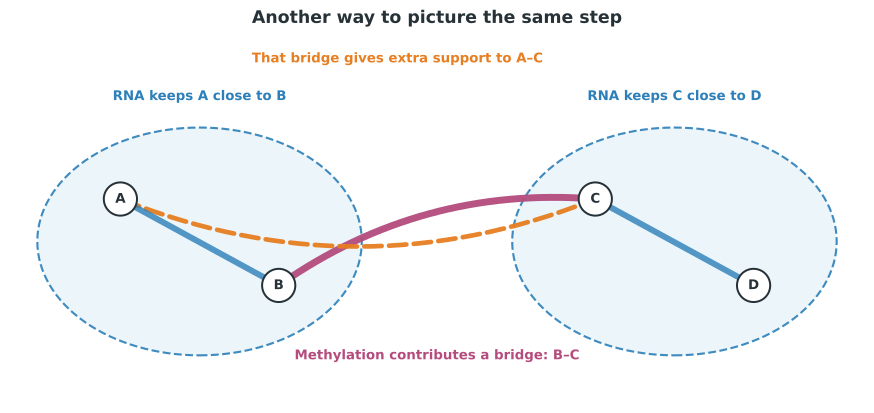
Methylation is therefore not placed directly on top of RNA. RNA keeps its local structure and uses methylation as additional evidence about how its local groups relate to each other.

The same update occurs in the other direction. Methylation keeps its strong local relationships and evaluates them using the current RNA view.

1.3 Repeating the process

After the first exchange, both networks have changed. RNA has listened to methylation, but methylation has also listened to RNA. If we stop after one round, each network has only heard the original version of the other one.

In the second round, they exchange their updated views. This allows information to move farther through the patient networks.

With four patients, the pattern is easier to see if we temporarily combine the two current views and hide very weak connections. The threshold is used only to keep the figure readable. It is not part of the SNF calculation.

Figure 1.5: The running combined patient network over several rounds. A-C and B-D become visible after the first exchange, and the same main links remain as later rounds settle down.

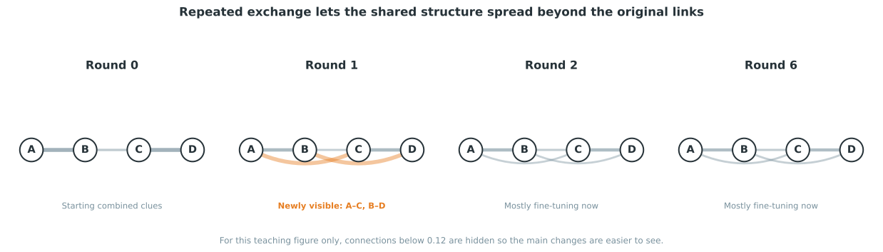
Round 0 contains the clues we started with: A-B from RNA, B-C from methylation and C-D from RNA. After the first exchange, A-C and B-D receive much more support. Later rounds mostly adjust the strength of those links rather than changing the overall picture again.

The changes do not all go in the same direction. Some original connections become weaker, while others become stronger. The networks redistribute their weights as information is exchanged.

Figure 1.6: Selected connection strengths over the exchange rounds. A-C strengthens quickly, A-D rises more slowly and stays weaker, while the original A-B relationship remains comparatively strong.

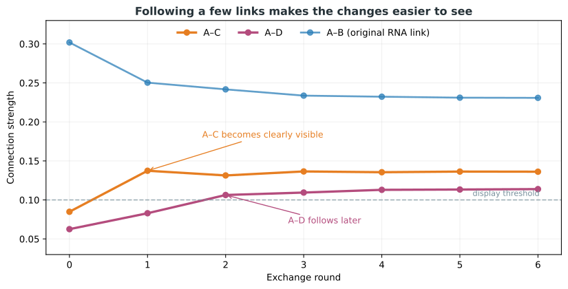
The plot shows that most of the change occurs early. Later rounds mainly fine-tune the network, so four snapshots are enough to show its development.

A few rounds are enough to show what changes here. In practice, SNF is usually run for more iterations. Twenty is a common software default, but it is a practical choice rather than a biologically meaningful number. We return to this point in the mathematics chapter.

1.4 The result of fusion

RNA and methylation remain separate networks during the exchange. After the last round, we still have an updated RNA view and an updated methylation view.

Those final views are then combined to give one fused patient-similarity network.

Figure 1.7: Final RNA and methylation networks are combined into one fused patient network.

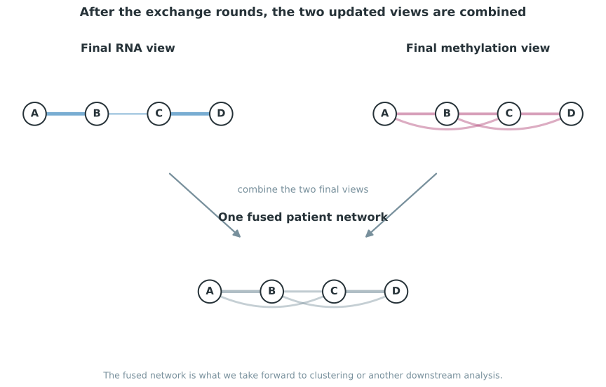
The fused network is the output from SNF. A strong connection between A and B means that the integrated analysis supports their similarity after the datasets have informed one another.

If we are interested in patient subtypes, we can cluster the fused network. Spectral clustering is commonly used for this purpose. Clustering comes after fusion and is separate from the exchange between networks.

So for now, keep the workflow in mind as:

measure the same patients in several ways → build one patient network per dataset → let the networks exchange information → combine the updated networks → analyse the fused network.

In the next chapter we will do this with a larger simulated study. After that, in the mathematics chapter, we will put names and equations on the network objects used in each step.