4 SNF exercises using real data
In the previous chapters, we used simulated data to explain how SNF works. We will now apply the method to a real multi-omics dataset. We will inspect each data layer, build and fuse the networks, cluster the patients, and examine how the results change with the parameters. The final exercise uses the fitted network to predict the subtype of new patients.
Each exercise contains a task, a short tip, and a collapsed solution with R and Python code. Try to complete the task before opening the solution. Small numerical differences may occur across software versions.
4.1 The dataset
We use breast.TCGA, a subset of The Cancer Genome Atlas breast cancer cohort. The dataset is distributed with the mixOmics package for its DIABLO tutorial (Singh et al. 2019, Bioinformatics, 35(17):3055–3062). We have exported the data to CSV files, so mixOmics and Bioconductor are not required for these exercises.
- 150 patients measured using three omics layers
- mRNA expression for 200 genes
- miRNA expression for 184 miRNAs
- protein abundance for 142 proteins measured by RPPA
- a PAM50 molecular subtype for each patient (Basal, Her2, or Luminal A)
- a test set of 70 additional patients for the final exercise, with mRNA and miRNA but no protein data
We use the subtype label only to evaluate the results. It is not used when the networks are constructed, fused, or clustered.
4.2 Downloading the data
Download the complete exercise dataset. The archive contains the training data used throughout the chapter and the test data used in the final exercise.
Extract the archive in the directory where you will run the R or Python code. It already contains a folder named data, so the resulting structure should look like this:
your-working-directory/
└── data/
    ├── exercise-mrna.csv
    ├── exercise-mirna.csv
    ├── exercise-protein.csv
    ├── exercise-patients.csv
    ├── exercise-mrna-test.csv
    ├── exercise-mirna-test.csv
    └── exercise-patients-test.csv
Run the code from your-working-directory, which is the directory containing the data folder. The file paths used below will then work without modification.
The files can also be downloaded separately:
- Training data: mRNA, miRNA, protein, and patient information
- Test data: mRNA, miRNA, and patient information
4.2.1 Setup
The exercises use SNFtool in R and snfpy in Python. The current snfpy release requires older versions of several scientific Python packages. Use the following command to create a compatible environment.
pip install "snfpy==0.2.2" "numpy<2" "scipy<1.13" "scikit-learn<1.8"library(SNFtool)
mrna <- read.csv("data/exercise-mrna.csv", row.names = 1, check.names = FALSE)
mirna <- read.csv("data/exercise-mirna.csv", row.names = 1, check.names = FALSE)
protein <- read.csv("data/exercise-protein.csv", row.names = 1, check.names = FALSE)
patients <- read.csv("data/exercise-patients.csv")
stopifnot(identical(rownames(mrna), rownames(mirna)))
stopifnot(identical(rownames(mrna), rownames(protein)))
stopifnot(identical(rownames(mrna), patients$Patient))
dim(mrna); dim(mirna); dim(protein)
table(patients$Subtype)[1] 150 200
[1] 150 184
[1] 150 142
Basal Her2 LumA
45 30 75import pandas as pd
from snf import compute
from sklearn.cluster import SpectralClustering
mrna = pd.read_csv("data/exercise-mrna.csv", index_col=0)
mirna = pd.read_csv("data/exercise-mirna.csv", index_col=0)
protein = pd.read_csv("data/exercise-protein.csv", index_col=0)
patients = pd.read_csv("data/exercise-patients.csv")
assert mrna.index.equals(mirna.index)
assert mrna.index.equals(protein.index)
assert mrna.index.tolist() == patients["Patient"].tolist()
print(mrna.shape, mirna.shape, protein.shape)
print(patients["Subtype"].value_counts())(150, 200) (150, 184) (150, 142)
Subtype
LumA 75
Basal 45
Her2 30
Name: count, dtype: int64The subtype groups have different sizes. There are 45 Basal, 30 Her2, and 75 Luminal A patients. Keep this imbalance in mind when interpreting the clustering results.
4.3 Exercise 1. Looking at the data before fusion
Task. Before running SNF, examine each omics layer separately. Make a two-dimensional PCA plot for the mRNA, miRNA, and protein data. Colour the patients by subtype. Does any one modality separate all three subtypes clearly?
Scale the variables before running PCA. You can use prcomp(scale(x)) in R or StandardScaler() before PCA() in Python. Plot the first two components and compare the amount of overlap among the three subtypes.
pca_mrna <- prcomp(scale(as.matrix(mrna)))$x[, 1:2]
pca_mirna <- prcomp(scale(as.matrix(mirna)))$x[, 1:2]
pca_protein <- prcomp(scale(as.matrix(protein)))$x[, 1:2]

subtype <- factor(patients$Subtype)
plot(pca_mrna, col = subtype, pch = 19, main = "mRNA")
plot(pca_mirna, col = subtype, pch = 19, main = "miRNA")
plot(pca_protein, col = subtype, pch = 19, main = "Protein")
import numpy as np
from sklearn.decomposition import PCA
from sklearn.preprocessing import StandardScaler
import matplotlib.pyplot as plt
def pca_2d(x):
return PCA(n_components=2).fit_transform(StandardScaler().fit_transform(x))
pca_mrna = pca_2d(mrna.to_numpy())
pca_mirna = pca_2d(mirna.to_numpy())
pca_protein = pca_2d(protein.to_numpy())
labels, colors = patients["Subtype"], patients["Subtype"].astype("category").cat.codes
fig, axes = plt.subplots(1, 3, figsize=(12, 4))
for ax, scores, title in zip(axes, [pca_mrna, pca_mirna, pca_protein], ["mRNA", "miRNA", "Protein"]):
ax.scatter(scores[:, 0], scores[:, 1], c=colors, cmap="Set1")
ax.set_title(title)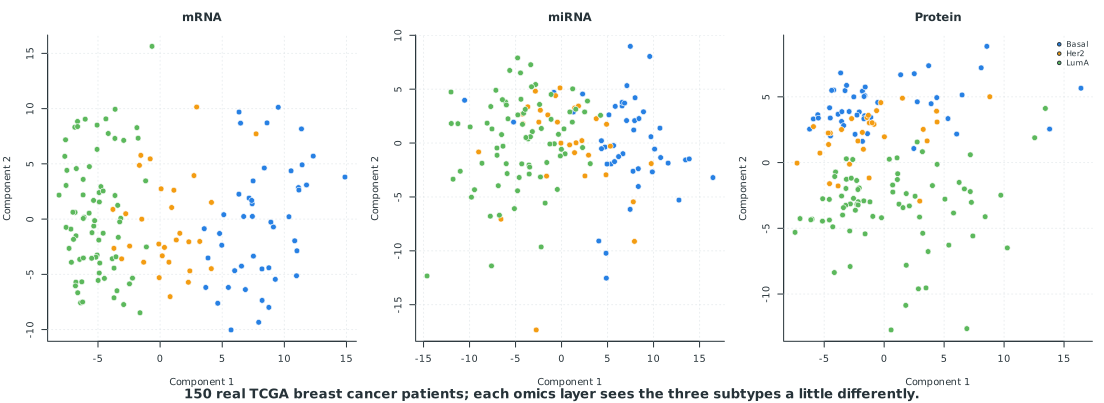
Basal is reasonably distinct in the mRNA data. Her2 and Luminal A overlap in all three modalities, and the separation is weakest in the miRNA data. This is not surprising because PAM50 subtypes were originally defined using gene-expression patterns. No single modality gives a clear separation of all three groups, so it is reasonable to examine whether fusion helps.
4.4 Exercise 2. Constructing one affinity network
Task. Standardize the mRNA data and construct its patient similarity network, \(W_{mRNA}\). Choose a reasonable value of K for 150 patients.
Values between 10 and 30 are often used as a starting range. We will begin with K = 15 and study the effect of changing it in Exercise 5.
K <- 15
sigma <- 0.5

mrna_z <- standardNormalization(as.matrix(mrna))
D_mrna <- sqrt(dist2(mrna_z, mrna_z))
W_mrna <- affinityMatrix(D_mrna, K = K, sigma = sigma)
dim(W_mrna)
[1] 150 150K = 15
mu = 0.5
W_mrna = compute.make_affinity(mrna.to_numpy(), metric="euclidean", K=K, mu=mu, normalize=True)
W_mrna.shape(150, 150)W_mrna is a 150 × 150 patient similarity network constructed from the 200 genes. The original gene dimension is no longer present. From this point onward, the analysis uses similarities between patients.
4.5 Exercise 3. Fusing the three networks
Task. Repeat Exercise 2 for the miRNA and protein data. Use the same K and kernel scale for all three modalities, and then fuse the networks using 20 iterations.
Both SNFtool::SNF() and compute.snf() can fuse more than two networks in one call. Pass all three affinity matrices together.
mirna_z <- standardNormalization(as.matrix(mirna))
protein_z <- standardNormalization(as.matrix(protein))
W_mirna <- affinityMatrix(sqrt(dist2(mirna_z, mirna_z)), K = K, sigma = sigma)
W_protein <- affinityMatrix(sqrt(dist2(protein_z, protein_z)), K = K, sigma = sigma)

W_fused <- SNF(list(W_mrna, W_mirna, W_protein), K = K, t = 20)
dim(W_fused)
max(abs(W_fused - t(W_fused)))
[1] 150 150
[1] 0affinities = compute.make_affinity(
mrna.to_numpy(), mirna.to_numpy(), protein.to_numpy(),
metric="euclidean", K=K, mu=mu, normalize=True,
)
W_mrna, W_mirna, W_protein = affinities
fused = compute.snf(*affinities, K=K, t=20)
fused.shape, abs(fused - fused.T).max()((150, 150), 0.0)The result is one 150 × 150 fused network. The symmetry check confirms that the similarity from patient (i) to patient (j) is the same as the similarity from (j) to (i).
4.6 Exercise 4. Clustering and comparison with the known subtypes
Task. Use the eigengap method to estimate the number of clusters in the fused network. Next, cluster the network into three groups because the dataset contains three known subtypes. Compare the inferred clusters with the subtype labels using the adjusted Rand index (ARI). Repeat the clustering for each individual modality.
Set affinity="precomputed" when using SpectralClustering because fused is already a similarity matrix. ARI can compare two partitions even when their cluster numbers differ.
estimateNumberOfClustersGivenGraph(W_fused, 2:6)

choose2 <- function(x) x * (x - 1) / 2
ari <- function(a, b) {
  tab <- table(a, b)
  obs <- sum(choose2(tab)); rp <- sum(choose2(rowSums(tab)))
  cp <- sum(choose2(colSums(tab))); tot <- choose2(sum(tab))
  exp <- rp * cp / tot
  (obs - exp) / ((rp + cp) / 2 - exp)
}

C <- 3
cl_mrna <- spectralClustering(W_mrna, K = C, type = 3)
cl_mirna <- spectralClustering(W_mirna, K = C, type = 3)
cl_protein <- spectralClustering(W_protein, K = C, type = 3)
cl_fused <- spectralClustering(W_fused, K = C, type = 3)

data.frame(
  Network = c("mRNA", "miRNA", "Protein", "Fused"),
  ARI = c(ari(cl_mrna, patients$Subtype), ari(cl_mirna, patients$Subtype),
          ari(cl_protein, patients$Subtype), ari(cl_fused, patients$Subtype))
)
table(Inferred = cl_fused, Truth = patients$Subtype)
$`Eigen-gap best`
[1] 2
$`Eigen-gap 2nd best`
[1] 4
Network ARI
1 mRNA 0.4056297
2 miRNA 0.3151206
3 Protein 0.4339528
4 Fused 0.4035045
Truth
Inferred Basal Her2 LumA
1 42 17 0
2 0 7 29
3 3 6 46first, second = compute.get_n_clusters(fused)
print(first, second)
def ari(a, b):
tab = pd.crosstab(pd.Series(a), pd.Series(b)).to_numpy()
c2 = lambda x: x * (x - 1) / 2
obs = c2(tab).sum(); rp = c2(tab.sum(1)).sum()
cp = c2(tab.sum(0)).sum(); tot = c2(tab.sum())
exp = rp * cp / tot
return (obs - exp) / ((rp + cp) / 2 - exp)
C = 3
cl_mrna = SpectralClustering(n_clusters=C, affinity="precomputed", random_state=1).fit_predict(W_mrna)
cl_mirna = SpectralClustering(n_clusters=C, affinity="precomputed", random_state=1).fit_predict(W_mirna)
cl_protein = SpectralClustering(n_clusters=C, affinity="precomputed", random_state=1).fit_predict(W_protein)
cl_fused = SpectralClustering(n_clusters=C, affinity="precomputed", random_state=1).fit_predict(fused)
for name, cl in [("mRNA", cl_mrna), ("miRNA", cl_mirna), ("Protein", cl_protein), ("Fused", cl_fused)]:
print(name, ari(cl, patients["Subtype"]))
print(pd.crosstab(cl_fused, patients["Subtype"], rownames=["Inferred"], colnames=["Truth"]))2 4
mRNA 0.40924611316819043
miRNA 0.3127454796592804
Protein 0.40884142516622757
Fused 0.4158487095416496
Truth Basal Her2 LumA
Inferred
0 42 17 0
1 3 6 49
2 0 7 26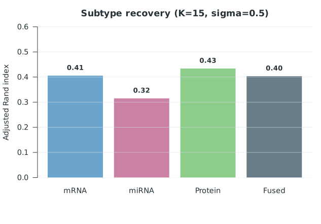
The eigengap method suggests two clusters, although the clinical variable contains three subtypes. This happens because the Basal group forms the clearest separation in the fused network, while Her2 and Luminal A are more difficult to distinguish.
The fused ARI is close to the best result from a single modality. In this dataset, the three modalities contain partly overlapping information about PAM50 subtype, so fusion does not produce a large improvement. SNF should therefore be compared with the individual networks in every analysis.
4.7 Exercise 5. Examining the parameters
Task. Repeat the fusion and clustering from Exercise 4 over a small parameter grid. Use K values of 10, 15, 20, and 30, and kernel scales of 0.3, 0.5, and 0.8. Record the fused ARI for every combination. How sensitive is the result to these choices?
Use two nested loops or construct a parameter grid. Keep t = 20 fixed so that only K and the kernel scale change.
results <- data.frame()
for (Kv in c(10, 15, 20, 30)) {
  for (sv in c(0.3, 0.5, 0.8)) {
    mw <- function(x) affinityMatrix(sqrt(dist2(standardNormalization(as.matrix(x)),
                                                 standardNormalization(as.matrix(x)))),
                                      K = Kv, sigma = sv)
    Wf <- SNF(list(mw(mrna), mw(mirna), mw(protein)), K = Kv, t = 20)
    cl <- spectralClustering(Wf, K = 3, type = 3)
    results <- rbind(results, data.frame(K = Kv, sigma = sv, ARI = ari(cl, patients$Subtype)))
  }
}
print(results)
K sigma ARI
1 10 0.3 0.4331797
2 10 0.5 0.4177544
3 10 0.8 0.4070732
4 15 0.3 0.4270833
5 15 0.5 0.4035045
6 15 0.8 0.3881714
7 20 0.3 0.4083333
8 20 0.5 0.3839286
9 20 0.8 0.3826484
10 30 0.3 0.4067935
11 30 0.5 0.3879310
12 30 0.8 0.3860294rows = []
for Kv in [10, 15, 20, 30]:
for mv in [0.3, 0.5, 0.8]:
aff = compute.make_affinity(mrna.to_numpy(), mirna.to_numpy(), protein.to_numpy(),
metric="euclidean", K=Kv, mu=mv, normalize=True)
wf = compute.snf(*aff, K=Kv, t=20)
cl = SpectralClustering(n_clusters=3, affinity="precomputed", random_state=1).fit_predict(wf)
rows.append({"K": Kv, "mu": mv, "ARI": ari(cl, patients["Subtype"])})
pd.DataFrame(rows) K mu ARI
0 10 0.3 0.434959
1 10 0.5 0.443807
2 10 0.8 0.442892
3 15 0.3 0.429000
4 15 0.5 0.415849
5 15 0.8 0.395279
6 20 0.3 0.425904
7 20 0.5 0.387019
8 20 0.8 0.392467
9 30 0.3 0.412649
10 30 0.5 0.383635
11 30 0.8 0.368072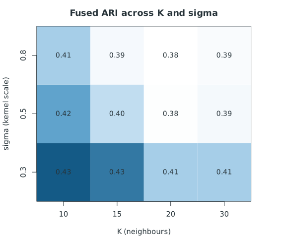
The ARI ranges from approximately 0.37 to 0.44. Smaller values of K and a narrower kernel perform slightly better for these data. The variation is noticeable but does not change the main conclusion from Exercise 4. None of the tested combinations gives a large improvement over the individual modalities.
4.8 Exercise 6. Predicting new patients
Task. Use the 150 training patients to predict the subtypes of the 70 test patients. Only mRNA and miRNA are available for the test set, so use these two modalities for both training and prediction. The true test labels are used only to calculate the final accuracy.
Use SNFtool::groupPredict() in R or compute.group_predict() in Python. These functions take the raw training and test feature matrices together with the training labels. They construct and fuse the required networks internally. The R function expects integer group labels, so convert the subtype names before calling it.
mrna_test <- read.csv("data/exercise-mrna-test.csv", row.names = 1, check.names = FALSE)
mirna_test <- read.csv("data/exercise-mirna-test.csv", row.names = 1, check.names = FALSE)
patients_test <- read.csv("data/exercise-patients-test.csv")

subtype_levels <- sort(unique(patients$Subtype))
groups_int <- as.integer(factor(patients$Subtype, levels = subtype_levels))

pred <- groupPredict(
  train = list(as.matrix(mrna), as.matrix(mirna)),
  test = list(as.matrix(mrna_test), as.matrix(mirna_test)),
  groups = groups_int, K = 15, alpha = 0.5, t = 20
)
# groupPredict() returns train+test concatenated; keep the test tail.
predicted_test <- subtype_levels[pred[(nrow(mrna) + 1):(nrow(mrna) + nrow(mrna_test))]]

mean(predicted_test == patients_test$Subtype)
table(Predicted = predicted_test, Truth = patients_test$Subtype)
[1] 0.9
Truth
Predicted Basal Her2 LumA
Basal 19 1 0
Her2 1 9 0
LumA 1 4 35mrna_test = pd.read_csv("data/exercise-mrna-test.csv", index_col=0)
mirna_test = pd.read_csv("data/exercise-mirna-test.csv", index_col=0)
patients_test = pd.read_csv("data/exercise-patients-test.csv")
subtype_levels = sorted(patients["Subtype"].unique())
label_to_int = {s: i for i, s in enumerate(subtype_levels)}
labels_int = patients["Subtype"].map(label_to_int).to_numpy()
# snfpy's group_predict returns predictions for the test subjects only.
predicted_int = compute.group_predict(
[mrna.to_numpy(), mirna.to_numpy()],
[mrna_test.to_numpy(), mirna_test.to_numpy()],
labels_int, K=15, mu=0.5, t=20,
)
predicted_test = [subtype_levels[i] for i in predicted_int]
print((pd.Series(predicted_test) == patients_test["Subtype"]).mean())
print(pd.crosstab(pd.Series(predicted_test, name="Predicted"), patients_test["Subtype"], colnames=["Truth"]))0.7428571428571429
Truth Basal Her2 LumA
Predicted
Basal 17 0 0
LumA 4 14 35The R implementation gives 90% accuracy on the test patients. The Python implementation gives 74% and does not assign any test patient to Her2. This difference is larger than we would expect from numerical rounding.
The two packages use different label-propagation procedures. SNFtool uses .csPrediction(), while snfpy uses _label_prop(). Therefore, the prediction results from the two implementations are not directly interchangeable. Package choice and version should be reported when this type of prediction is used.
4.9 Wrapping up
In these exercises, we applied the complete SNF workflow to a real dataset. We inspected the individual modalities, constructed and fused their networks, compared the clusters with known subtypes, examined the main parameters, and predicted labels for new patients.
Fusion did not clearly outperform the best individual modality for unsupervised clustering. The supervised label-propagation exercise performed better, although the R and Python implementations gave different results. These comparisons show why the individual networks, parameter sensitivity, and software implementation should all be examined when reporting an SNF analysis.