3 Math behind Similarity Network Fusion
We have seen the steps of SNF. Each dataset gives a patient network. The networks exchange information through local neighbours, and their updated views are combined after several rounds.
3.1 Starting from the data matrix
For one data type we write the data as
\[X\in\mathbb{R}^{n\times p},\]
where \(n\) is the number of patients and \(p\) is the number of measured variables.
For RNA, the columns may be genes. For methylation, they may be CpG sites. The datasets do not need to have the same number of columns, but they must contain the same patients in their rows.
The RNA data use only two variables so that the patients can be drawn:
| Patient | RNA feature 1 | RNA feature 2 |
|---|---|---|
| A | 0.00 | 0.00 |
| B | 0.40 | 0.10 |
| C | 2.60 | 0.10 |
| D | 3.00 | 0.00 |
A and B are close to each other, while B and C are far apart. We calculate these two distances below.
3.2 Patient-to-patient distance
Using Euclidean distance,
\[d_{ij}=\sqrt{\sum_{r=1}^{p}(x_{ir}-x_{jr})^2}.\]
For A and B,
\[d_{AB} = \sqrt{(0-0.40)^2+(0-0.10)^2} \approx0.41.\]
For B and C,
\[d_{BC} = \sqrt{(0.40-2.60)^2+(0.10-0.10)^2} =2.20.\]
In RNA space, A and B are therefore much closer than B and C.
The choice of distance measure determines what similarity means in the analysis. SNF can use other distance measures, but the choice should be appropriate for the data and its preprocessing.
3.3 Similarity network W
We now have two RNA distances: \(d_{AB}\approx0.41\) and \(d_{BC}=2.20\). A is close to B, whereas B is far from C.
A small distance means that two patients are similar in this modality. In a similarity network, a strong connection should have a large value and a weak connection should have a small value. Distance runs in the opposite direction. A small distance should therefore produce a large connection strength, and a large distance should produce a small one.
\[\text{small distance }d_{ij}\quad\Longrightarrow\quad\text{large connection strength},\]
\[\text{large distance }d_{ij}\quad\Longrightarrow\quad\text{small connection strength}.\]
Before the distances can form a similarity network, this direction must be reversed. SNF converts each distance to an affinity, which increases as the patients become closer. The matrix containing all pairwise affinities for one modality is called \(W\). The entry \(W_{ij}\) is the initial connection strength between patients \(i\) and \(j\) in that modality.
We construct one \(W\) for RNA and another for methylation, using the data from each modality. The modalities do not need the same number or type of features. RNA may contain thousands of genes, while methylation may contain hundreds of thousands of CpG sites. Once the distances have been converted to affinities, however, \(W_{RNA}\) and \(W_{Meth}\) are both \(n\times n\) patient-by-patient matrices. Here, \(n=4\). Datasets with different features have therefore been converted to matrices with the same dimensions, which allows them to be combined.
3.3.1 Why one global distance scale is not enough
One possible conversion would use a fixed rule for every patient, such as treating any distance below 1 as a strong connection. This is problematic when patients are not distributed evenly. Suppose one patient lies in a crowded region, where its nearest neighbours are close together, while another lies in a sparse region, where even its nearest neighbours are relatively far away. A distance of 1 may be unremarkable in the crowded region because many patients are that close. The same distance may represent a close pair in the sparse region. A single fixed scale cannot represent both situations well.
SNF therefore evaluates each distance relative to the local neighbourhoods of the two patients involved, rather than using one scale for the dataset.
3.3.2 Building a local scale
The same raw distance can have a different meaning in different parts of the data.
Consider two patients separated by a distance of \(1\). In a crowded part of the data, where nearby patients are only \(0.2\) or \(0.3\) apart, this distance is relatively large. In a sparse region, where nearby patients are usually \(2\) or \(3\) apart, the same distance is relatively small.
SNF accounts for this difference by estimating a typical nearby distance for each patient.
For patient \(i\), we find the \(K\) nearest other patients and calculate their mean distance from \(i\). We denote this mean by \(\bar d_i\).
A small \(\bar d_i\) indicates that patient \(i\) lies in a crowded region. A large \(\bar d_i\) indicates that the nearby patients are more spread out.
For a pair of patients, \(i\) and \(j\), we need one local scale that describes the distances around them.
SNF combines three quantities:
- the typical nearby distance around patient \(i\), \(\bar d_i\)
- the typical nearby distance around patient \(j\), \(\bar d_j\)
- the observed distance between the two patients, \(d_{ij}\)
Their average defines the local scale:
\[ \tau_{ij} = \sigma \frac{\bar d_i+\bar d_j+d_{ij}}{3}. \]
The result, \(\tau_{ij}\), is the local scale for the pair \(i,j\). It provides a reference for interpreting their distance.
If \(\tau_{ij}\) is small, then distances around this pair are generally small, so even a moderate value of \(d_{ij}\) may represent a meaningful separation.
If \(\tau_{ij}\) is large, then distances around this pair are generally larger, so the same value of \(d_{ij}\) may still indicate that the two patients are relatively close.
The parameter \(\sigma\) controls the size of the local scales. Increasing \(\sigma\) makes all \(\tau_{ij}\) values larger, while decreasing it makes them smaller. Together with \(K\), it is one of the settings used in SNF.
SNF therefore does not determine whether two patients are close from \(d_{ij}\) alone. It asks:
Is this distance small or large compared with the distances that are normal around these two patients?
The local scale \(\tau_{ij}\) provides the reference needed to answer this question.
3.3.3 Turning distance into affinity
Once \(\tau_{ij}\) has been calculated, the observed distance \(d_{ij}\) can be compared with the local scale for that pair.
The relevant quantity is
\[ \frac{d_{ij}}{\tau_{ij}}. \]
This ratio is the distance between the two patients relative to their local neighbourhood.
Suppose that two pairs of patients both have
\[ d_{ij}=1. \]
For the first pair, suppose
\[ \tau_{ij}=0.5. \]
Then
\[ \frac{d_{ij}}{\tau_{ij}} = \frac{1}{0.5} = 2. \]
Their distance is twice the local scale. Relative to the distances around them, these patients are far apart.
For the second pair, suppose
\[ \tau_{ij}=2. \]
Then
\[ \frac{d_{ij}}{\tau_{ij}} = \frac{1}{2} = 0.5. \]
Their distance is half the local scale. Relative to their neighbourhood, these patients are close.
This local comparison allows SNF to handle crowded and sparse regions differently. A distance of \(1\) does not have to carry the same meaning throughout the dataset.
The relative distance is then converted to an affinity, which describes the strength of the connection between the two patients.
SNF uses
\[ W_{ij} = \frac{1}{\sqrt{2\pi}\tau_{ij}} \exp\left( -\frac{1}{2} \left( \frac{d_{ij}}{\tau_{ij}} \right)^2 \right). \]
The expression can also be written as
\[ W_{ij} = \frac{1}{\sqrt{2\pi}\tau_{ij}} \exp\left( -\frac{d_{ij}^2}{2\tau_{ij}^2} \right). \]
The two formulas are equivalent. The first form makes the relative distance
\[ \frac{d_{ij}}{\tau_{ij}} \]
explicit.
First, consider the exponential term:
\[ \exp\left( -\frac{1}{2} \left( \frac{d_{ij}}{\tau_{ij}} \right)^2 \right). \]
If \(d_{ij}\) is small compared with \(\tau_{ij}\), then
\[ \frac{d_{ij}}{\tau_{ij}} \]
is close to \(0\).
For example, if
\[ \frac{d_{ij}}{\tau_{ij}}=0, \]
then the exponential part becomes
\[ \exp(0)=1. \]
The connection is therefore strongest when the two patients are close.
As \(d_{ij}\) increases relative to \(\tau_{ij}\), the ratio becomes larger.
For example, if
\[ \frac{d_{ij}}{\tau_{ij}}=1, \]
then
\[ \exp\left(-\frac{1}{2}\right) \approx 0.61. \]
If
\[ \frac{d_{ij}}{\tau_{ij}}=2, \]
then
\[ \exp(-2) \approx 0.14. \]
If
\[ \frac{d_{ij}}{\tau_{ij}}=3, \]
then
\[ \exp(-4.5) \approx 0.011. \]
The affinity therefore decreases quickly when two patients are far apart relative to their local neighbourhood.
Squaring the ratio,
\[ \left( \frac{d_{ij}}{\tau_{ij}} \right)^2, \]
makes the decrease stronger as the relative distance grows. The exponential function converts the result to a similarity that decreases smoothly.
The remaining factor
\[ \frac{1}{\sqrt{2\pi}\tau_{ij}} \]
comes from the Gaussian function.
The Gaussian has the bell-shaped form used throughout statistics. Its width is controlled by \(\tau_{ij}\). A small \(\tau_{ij}\) produces a narrow curve, while a large value produces a wider curve.
Changing the width also changes the height of the Gaussian. This is why \(\tau_{ij}\) appears both inside and outside the exponential.
Inside the exponential,
\[ \frac{d_{ij}}{\tau_{ij}} \]
determines how large the distance is relative to the local neighbourhood.
Outside the exponential,
\[ \frac{1}{\sqrt{2\pi}\tau_{ij}} \]
adjusts the height of the Gaussian to match that same scale.
The values \(2\), \(\pi\) and the square root are fixed parts of the Gaussian formula rather than parameters chosen for the analysis.
The conversion is
\[ \text{raw distance} \quad\longrightarrow\quad \text{distance relative to the local neighbourhood} \quad\longrightarrow\quad \text{affinity}. \]
First, \(\tau_{ij}\) describes the typical distances around the pair.
Then
\[ \frac{d_{ij}}{\tau_{ij}} \]
shows whether the observed distance is small or large relative to the local scale.
Finally, the exponential function converts the relative distance to a connection strength. The value is large when the patients are locally close and small when they are locally far apart.
For the RNA data below, A and B have
\[ \tau_{AB}\approx0.86, \]
while B and C have
\[ \tau_{BC}\approx1.28. \]
The local scale for B and C is larger because the distances around that pair are larger. The observed distance \(d_{BC}\) also contributes directly to \(\tau_{BC}\).
SNF considers more than whether \(d_{AB}\) is smaller than \(d_{BC}\). Each distance is evaluated relative to the local structure around that pair.
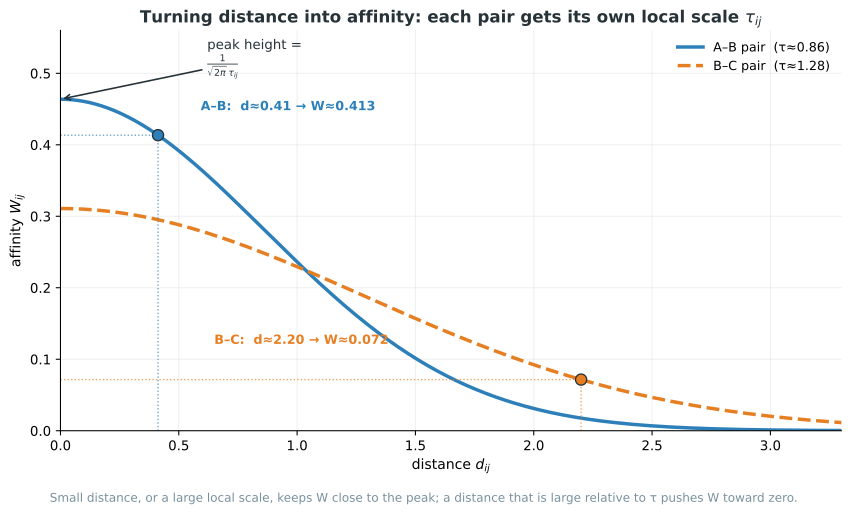
A-B has a raw distance of \(0.41\) and a local scale of \(\tau_{AB}=0.86\). The distance between A and B is therefore less than half the local scale for this pair:
\[ \frac{0.41}{0.86}\approx0.48. \]
A and B are close relative to the distances around them. On the Gaussian curve for A-B, they lie close to the peak and have a relatively large affinity:
\[ W_{AB}\approx0.413. \]
For B-C, the raw distance is \(2.20\) and the local scale is \(\tau_{BC}=1.28\):
\[ \frac{2.20}{1.28}\approx1.72. \]
The distance between B and C is about \(1.7\) times their local scale. Relative to the distances around this pair, B and C are much farther apart. On the Gaussian curve for B-C, they lie farther from the peak, where the curve has already dropped substantially:
\[ W_{BC}\approx0.072. \]
Both affinities use the same formula. The value that changes between pairs is \(\tau_{ij}\). SNF calculates this local scale separately for every pair, so each raw distance is interpreted relative to its neighbourhood.
The original SNF paper (Wang et al., 2014) writes this step as a single exponential kernel controlled by one hyperparameter. The implementation in SNFtool, which is followed in this chapter, computes the Gaussian density shown above and uses the sigma parameter. Both approaches compare a distance with a local neighbourhood scale, but their equations are not algebraically identical. When comparing implementations or reading the original paper, it is therefore necessary to check which convention is being used.
3.3.4 Calculate W in R and Python
source("scripts/toy-snf-helpers.R")

rna <- rbind(A = c(0, 0), B = c(0.40, 0.10),
             C = c(2.60, 0.10), D = c(3, 0))

W_rna <- affinity_from_points(rna, K = 2, sigma = 0.8)
round(W_rna, 3)
A B C D
A 0.496 0.413 0.054 0.043
B 0.413 0.573 0.072 0.054
C 0.054 0.072 0.573 0.413
D 0.043 0.054 0.413 0.496import numpy as np
from scripts.toy_snf_helpers import affinity_from_points
rna = np.array([[0, 0], [0.40, 0.10], [2.60, 0.10], [3, 0]])
W_rna = affinity_from_points(rna, K=2, sigma=0.8)
print(np.round(W_rna, 3))[[0.496 0.413 0.054 0.043]
[0.413 0.573 0.072 0.054]
[0.054 0.072 0.573 0.413]
[0.043 0.054 0.413 0.496]]The numerical result follows the geometry of the RNA data. The A-B affinity is 0.413, while the B-C affinity is 0.072. A is close to B and B is far from C, as shown in the first chapter. The same calculation is performed separately for methylation using its coordinates and distances. At this stage, RNA and methylation still have separate \(4\times4\) networks. No information has been exchanged.
3.4 P puts each network on a common scale
The next step places each modality’s network on a common scale before RNA and methylation exchange information.
\(W_{RNA}\) and \(W_{Meth}\) can have different numerical ranges. Differences in the number of variables, noise levels and distance distributions may make the raw affinities in one modality larger than those in another, even when that modality is not more informative. If the raw values were used directly, the modality with larger values could dominate the update. SNF avoids this problem by normalizing every row of \(W\) to a fixed total. The resulting matrix is called \(P\).
The effect of this normalization can be seen by working through one row.
3.4.1 Normalizing one row by hand
For illustration, suppose patient A has the following raw affinities to the other three patients:
\[W_{AB}=0.80,\qquad W_{AC}=0.15,\qquad W_{AD}=0.05.\]
These values add to \(0.80+0.15+0.05=1.00\), which makes the arithmetic easy to follow. The values in our four-patient data do not add up this neatly, and we return to them below.
The normalization of one row has two parts:
- Patient A keeps half of the row weight, so \(P_{AA}=0.50\).
- The remaining half is divided among B, C and D in proportion to their raw affinities.
Because the raw affinities for B, C and D add to \(1.00\), the proportional allocation is obtained by multiplying each value by \(0.50\):
\[P_{AB}=0.50\times\frac{0.80}{1.00}=0.40, \qquad P_{AC}=0.50\times\frac{0.15}{1.00}=0.075, \qquad P_{AD}=0.50\times\frac{0.05}{1.00}=0.025.\]
The row is
\[P_A=[\,0.50,\;0.40,\;0.075,\;0.025\,].\]
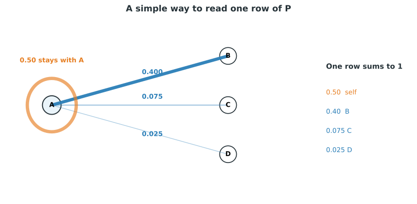
By construction, the row sums to 1: \(0.50+0.40+0.075+0.025=1\).
3.4.2 Interpreting P_AB = 0.40
\(P_{AB}=0.40\) does not mean that A and B are 40% biologically similar. It is not a biological percentage. It means that 0.40 of the available weight in patient A’s normalized row is assigned to B. In general:
\(P\) describes how each sample distributes its network weight across itself and the other samples.
Patient B receives much more of A’s row weight than C or D because B had the largest raw affinity.
3.4.3 The general formula
For any pair \(i,j\), the same rule is written as
\[P_{ij}= \begin{cases} \dfrac{W_{ij}}{2\sum_{k\neq i}W_{ik}}, & i\neq j,\\[8pt] \dfrac12, & i=j. \end{cases}\]
The denominator \(2\sum_{k\neq i}W_{ik}\) implements the two parts of the normalization. Dividing by twice the off-diagonal row total allocates half of the row weight across the off-diagonal entries in proportion to their affinities. The other half remains on the diagonal.
Normalizing row A gives the A-to-B value, while normalizing row B gives the B-to-A value. The row totals are generally different, so these two values may not agree. SNF restores symmetry by averaging the row-normalized matrix with its transpose, \(P\leftarrow(P+P^{\mathsf T})/2\). This makes \(P_{AB}\) and \(P_{BA}\) identical. The \(P_{RNA}\) matrix below therefore includes both row normalization and this averaging step.
3.4.4 Applying the normalization to our example
We now apply the row normalization and symmetry step to the RNA and methylation \(W\) matrices from the previous section.
source("scripts/toy-snf-helpers.R")

rna  <- rbind(A = c(0, 0), B = c(0.40, 0.10), C = c(2.60, 0.10), D = c(3, 0))
meth <- rbind(A = c(0, 0), B = c(1.25, 0.10), C = c(1.75, -0.10), D = c(3, 0))

W_rna  <- affinity_from_points(rna,  K = 2, sigma = 0.8)
W_meth <- affinity_from_points(meth, K = 2, sigma = 0.8)

P_rna  <- normalise_P(W_rna)
P_meth <- normalise_P(W_meth)
round(P_rna, 3)
round(P_meth, 3)
> round(P_rna, 3)
A B C D
A 0.500 0.394 0.052 0.042
B 0.394 0.500 0.066 0.052
C 0.052 0.066 0.500 0.394
D 0.042 0.052 0.394 0.500
> round(P_meth, 3)
A B C D
A 0.500 0.199 0.115 0.066
B 0.199 0.500 0.305 0.115
C 0.115 0.305 0.500 0.199
D 0.066 0.115 0.199 0.500import numpy as np
from scripts.toy_snf_helpers import affinity_from_points, normalise_P
rna = np.array([[0, 0], [0.40, 0.10], [2.60, 0.10], [3, 0]])
meth = np.array([[0, 0], [1.25, 0.10], [1.75, -0.10], [3, 0]])
W_rna = affinity_from_points(rna, K=2, sigma=0.8)
W_meth = affinity_from_points(meth, K=2, sigma=0.8)
P_rna = normalise_P(W_rna)
P_meth = normalise_P(W_meth)
print(np.round(P_rna, 3))
print(np.round(P_meth, 3))[[0.5 0.394 0.052 0.042]
[0.394 0.5 0.066 0.052]
[0.052 0.066 0.5 0.394]
[0.042 0.052 0.394 0.5 ]]
[[0.5 0.199 0.115 0.066]
[0.199 0.5 0.305 0.115]
[0.115 0.305 0.5 0.199]
[0.066 0.115 0.199 0.5 ]]Row A of \(P_{RNA}\) has the same pattern as \(W_{RNA}\). Patient B receives the largest share, 0.394, while C and D receive 0.052 and 0.042. Row B of \(P_{Meth}\) shows a different pattern. Patient C receives the largest share, 0.305, reflecting the strong B-C connection in methylation. These values are used again below.
3.4.5 W is fixed while P changes
The two matrices have different roles:
- \(W\) is the initial affinity network. It is constructed once from the distances and remains fixed.
- \(P\) is initialized from the normalized \(W\) and is repeatedly updated as RNA and methylation exchange information.
This produces one \(P\) for each round of exchange:
\[P^{(0)}\rightarrow P^{(1)}\rightarrow P^{(2)}\rightarrow\cdots\]
\(P^{(0)}\) is the normalized matrix calculated above. The next two sections show how \(P^{(1)}\) is calculated from \(P^{(0)}\).
3.5 S keeps the local neighbours
\(P\) describes the current network. Each patient’s row contains a weight for every other patient, including weak connections to distant patients. During the exchange step, each modality should rely on its stronger local relationships rather than its weakest connections.
SNF therefore constructs a second matrix for each modality, called \(S\). The matrix \(P\) represents the current network. The matrix \(S\) identifies the nearby samples used to represent each patient during the exchange.
\(S\) is constructed by retaining the \(K\) largest entries in each row of \(P\) and setting the remaining entries to zero. This is the same \(K\) used earlier for the local distance scale. The retained entries are then rescaled so that the row sums to 1.
3.5.1 Calculating the row for patient A
Row A of the RNA \(P\) matrix is
\[P_A=[\,0.500,\;0.394,\;0.052,\;0.042\,].\]
With \(K=2\), we retain the two largest entries in this row and set the others to zero. From largest to smallest, the entries are \(0.500\text{ (A itself)},\ 0.394\text{ (B)},\ 0.052\text{ (C)},\ 0.042\text{ (D)}\). The values for A and B are retained, while those for C and D are set to zero.
Patient A’s diagonal entry, \(P_{AA}=0.5\), is retained because it is one of the two largest values in the row. This follows from the normalization rather than from these particular values. Since the off-diagonal entries share the other half of the row weight, \(P_{ii}=0.5\) is at least as large as any individual off-diagonal entry. The diagonal is therefore usually among the entries retained in \(S\).
The two retained values are renormalized to sum to 1:
\[S_{AA}=\frac{0.500}{0.500+0.394}\approx0.559, \qquad S_{AB}=\frac{0.394}{0.500+0.394}\approx0.441, \qquad S_{AC}=S_{AD}=0.\]
The A row of \(S_{RNA}\) is therefore
\[S_A=[\,0.559,\;0.441,\;0,\;0\,].\]
3.5.2 Interpreting this row
The row \([0.559,\,0.441,\,0,\,0]\) does not describe a new patient made by mixing 55.9% of patient A’s RNA measurements with 44.1% of patient B’s measurements. The original gene-expression values are not averaged or combined at this stage.
The row describes influence in the calculation. When patient A’s local RNA neighbourhood is used, A receives a weight of 0.559 and B receives a weight of 0.441. Patients C and D receive zero weight.
For the remainder of the chapter, we use the following shorthand for A’s RNA neighbourhood:
\[0.559A+0.441B,\]
This means that A contributes a weight of 0.559, B contributes 0.441, and C and D contribute zero when A’s local RNA neighbourhood is used. The “+” sign does not indicate addition of the original measurements. It provides a compact notation for the neighbourhood weights.
3.5.3 Calculating the row for patient C
Row C of \(P_{RNA}\) is \([\,0.052,\;0.066,\;0.500,\;0.394\,]\). The two largest entries are C itself, with 0.500, and D, with 0.394. Renormalization gives the same weights as for A because the coordinates have a mirror symmetry between the A/B and C/D pairs:
\[S_C=[\,0,\;0,\;0.559,\;0.441\,], \qquad\text{read as}\qquad 0.559C+0.441D.\]
The next section uses these two RNA neighbourhoods:
\[\text{RNA neighbourhood of A: } 0.559A+0.441B \qquad\qquad \text{RNA neighbourhood of C: } 0.559C+0.441D.\]
3.5.4 The different roles of P and S
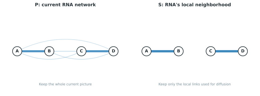
- \(P_{RNA}\) contains the current RNA network, including weak connections.
- \(S_{RNA}\) contains the nearby RNA samples used to represent each patient during the exchange.
\(S\) is constructed once from the initial \(P\) and remains fixed for the rest of the calculation. In contrast, \(P\) changes after every round as RNA and methylation exchange information. The next section uses this distinction.
The original SNF paper defines \(S\) directly from the raw affinities \(W\). For patient \(i\), let \(\mathcal N_i\) contain its \(K\) nearest other patients, excluding \(i\) itself. Then
\[S_{ij}^{\text{paper}}= \begin{cases} \dfrac{W_{ij}}{\sum_{k\in\mathcal N_i}W_{ik}}, & j\in\mathcal N_i,\\[8pt] 0, & \text{otherwise.} \end{cases}\]
The implementation in SNFtool, and the helper code used in this chapter, instead constructs the local matrix from the row-normalized \(P\). It includes the diagonal when selecting the \(K\) largest entries:
\[S_{ij}= \begin{cases} \dfrac{P_{ij}}{\sum_{k\in\mathcal N_i}P_{ik}}, & j\in\mathcal N_i,\\[8pt] 0, & \text{otherwise}, \end{cases} \qquad \mathcal N_i=\{\,K\text{ largest entries of row }i\text{ of }P,\text{ including }i\text{ itself}\,\}.\]
This is why patient A’s diagonal entry, \(S_{AA}=0.559\), is retained together with its strongest neighbour. The matrix does not contain only off-diagonal neighbours. Both definitions retain and normalize a small local neighbourhood, but their formulas are different. This chapter follows the software convention because it matches the calculations produced by the code.
3.6 One RNA update using methylation
We now calculate the RNA connection between patients A and C after one update from methylation.
From the previous section, patient A’s local RNA neighbourhood is represented by \(0.559A+0.441B\), and patient C’s by \(0.559C+0.441D\).
The update examines how strongly methylation connects every member of A’s RNA neighbourhood with every member of C’s RNA neighbourhood. A’s neighbourhood contains A and B, while C’s contains C and D. There are therefore four cross-neighbourhood comparisons: A with C, A with D, B with C and B with D.
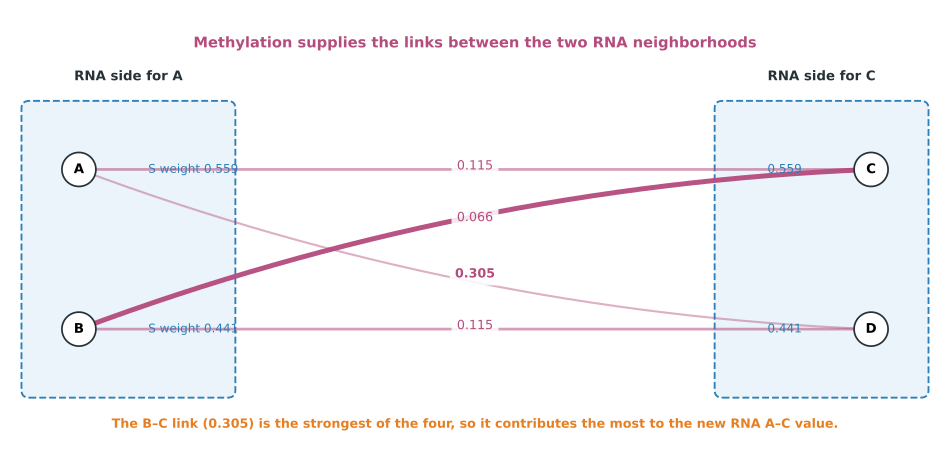
The current methylation network, \(P_{Meth}\), contains the strengths of these four relationships. These are the values calculated in the previous section:
\[P_{Meth}(A,C)=0.115, \qquad P_{Meth}(A,D)=0.066, \qquad P_{Meth}(B,C)=0.305, \qquad P_{Meth}(B,D)=0.115.\]
3.6.1 Four contributions
Each methylation relationship is combined with the RNA neighbourhood weights on both sides.
Term 1: A with C
\[0.559\times0.115\times0.559\approx0.036.\]
Reading the factors from left to right, the first \(0.559\) is A’s weight in its RNA neighbourhood. The value \(0.115\) is the current A-C connection in methylation. The final \(0.559\) is C’s weight in its RNA neighbourhood. This term follows the path start at A, use the methylation A-C relationship, and finish at C. It is the contribution of the direct methylation A-C relationship to the updated RNA A-C value.
Term 2: A with D
\[0.559\times0.066\times0.441\approx0.016.\]
The first \(0.559\) is again A’s weight. The value \(0.066\) is the methylation A-D relationship, and \(0.441\) is D’s weight in C’s RNA neighbourhood. This term follows the path start at A, use the methylation A-D relationship, and finish at D. The A-D relationship contributes to the update for C because RNA includes D in C’s trusted local neighbourhood.
Term 3: B with C
\[0.441\times0.305\times0.559\approx0.075.\]
Here, \(0.441\) is B’s weight in A’s RNA neighbourhood, \(0.305\) is the methylation B-C relationship, and \(0.559\) is C’s weight in its RNA neighbourhood. The B-C relationship is the strongest of the four, so this is the largest term. RNA treats B as a close local neighbour of A. When methylation gives B and C a strong connection, that evidence contributes to the RNA relationship between A and C. The methylation B-C value is not directly copied to A-C. It is one of four contributions to the weighted comparison between the two RNA neighbourhoods.
Term 4: B with D
\[0.441\times0.115\times0.441\approx0.022.\]
The first \(0.441\) is B’s weight in A’s RNA neighbourhood. The value \(0.115\) is the methylation B-D relationship, and the final \(0.441\) is D’s weight in C’s RNA neighbourhood. This term follows the path start at B, use the methylation B-D relationship, and finish at D.
Every one of the four terms has the same shape:
\[\underbrace{\text{RNA weight of a neighbour of A}}_{\text{first factor}} \ \times\ \underbrace{\text{methylation's connection between that neighbour and one of C's}}_{\text{middle factor}} \ \times\ \underbrace{\text{RNA weight of that neighbour of C}}_{\text{last factor}}\]
The first factor gives the weight of a sample in A’s RNA neighbourhood. The middle factor gives the methylation connection between the two samples. The last factor gives the weight of the second sample in C’s RNA neighbourhood. Their product is the contribution from one path. Adding the four paths gives the total.
3.6.2 Adding the four contributions
\[\tilde P_{RNA}^{(1)}(A,C)\approx0.036+0.016+0.075+0.022=0.150.\]
We denote this result by \(\tilde P\), rather than \(P^{(1)}\), because it has not yet been normalized. The normalization required before the next round is described at the end of this section.
source("scripts/toy-snf-helpers.R")

rna  <- rbind(A = c(0, 0), B = c(0.40, 0.10), C = c(2.60, 0.10), D = c(3, 0))
meth <- rbind(A = c(0, 0), B = c(1.25, 0.10), C = c(1.75, -0.10), D = c(3, 0))

P_rna  <- normalise_P(affinity_from_points(rna,  K = 2, sigma = 0.8))
P_meth <- normalise_P(affinity_from_points(meth, K = 2, sigma = 0.8))
S_rna  <- trusted_S(P_rna, K = 2)

term1 <- S_rna["A","A"] * P_meth["A","C"] * S_rna["C","C"]
term2 <- S_rna["A","A"] * P_meth["A","D"] * S_rna["C","D"]
term3 <- S_rna["A","B"] * P_meth["B","C"] * S_rna["C","C"]
term4 <- S_rna["A","B"] * P_meth["B","D"] * S_rna["C","D"]

round(c(term1 = term1, term2 = term2, term3 = term3, term4 = term4), 3)
round(sum(term1, term2, term3, term4), 3)
term1 term2 term3 term4
0.036 0.016 0.075 0.022
[1] 0.15import numpy as np
from scripts.toy_snf_helpers import affinity_from_points, normalise_P, trusted_S
rna = np.array([[0, 0], [0.40, 0.10], [2.60, 0.10], [3, 0]])
meth = np.array([[0, 0], [1.25, 0.10], [1.75, -0.10], [3, 0]])
labels = ["A", "B", "C", "D"]
P_rna = normalise_P(affinity_from_points(rna, K=2, sigma=0.8))
P_meth = normalise_P(affinity_from_points(meth, K=2, sigma=0.8))
S_rna = trusted_S(P_rna, K=2)
def idx(lab): return labels.index(lab)
term1 = S_rna[idx("A"), idx("A")] * P_meth[idx("A"), idx("C")] * S_rna[idx("C"), idx("C")]
term2 = S_rna[idx("A"), idx("A")] * P_meth[idx("A"), idx("D")] * S_rna[idx("C"), idx("D")]
term3 = S_rna[idx("A"), idx("B")] * P_meth[idx("B"), idx("C")] * S_rna[idx("C"), idx("C")]
term4 = S_rna[idx("A"), idx("B")] * P_meth[idx("B"), idx("D")] * S_rna[idx("C"), idx("D")]
print(np.round([term1, term2, term3, term4], 3))
print(round(term1 + term2 + term3 + term4, 3))[0.036 0.016 0.075 0.022]
0.153.6.3 Double sum
The four terms have the same structure and can be written as one expression covering every pairing. Let \(a\) denote one of A’s retained RNA neighbours, so \(a\) can be A or B. Let \(b\) denote one of C’s retained RNA neighbours, so \(b\) can be C or D. Then
\[\tilde P_{RNA}(A,C)=\sum_{a}\sum_{b}S_{RNA}(A,a)\,P_{Meth}(a,b)\,S_{RNA}(C,b).\]
The two sums mean that every allowed neighbour \(a\) on the A side is paired with every allowed neighbour \(b\) on the C side. For each pair, the three factors are multiplied, and the products are then added. With \(a\in\{A,B\}\) and \(b\in\{C,D\}\), this gives the same four terms calculated above.
The same expression applies to any pair of patients \(i\) and \(j\):
\[\tilde P_{RNA}(i,j)=\sum_{a}\sum_{b}S_{RNA}(i,a)\,P_{Meth}(a,b)\,S_{RNA}(j,b).\]
Here, \(i\) and \(j\) are the patients whose relationship is being updated. The index \(a\) ranges over the retained RNA neighbours of \(i\), while \(b\) ranges over the retained RNA neighbours of \(j\).
3.6.4 Matrix multiplication
Writing a separate sum for every pair becomes impractical with more than four patients. Matrix multiplication performs all pairwise calculations at once:
\[\tilde P_{RNA}=S_{RNA}\,P_{Meth}\,S_{RNA}^{\mathsf T}.\]
The role of the transpose can be seen from the \((A,C)\) entry. Matrix multiplication takes row A from the matrix on the left and column C from the matrix on the right, multiplies the corresponding values and adds the products. Row A of \(S_{RNA}\) contains the neighbourhood weights already calculated for A:
\[\text{row A of }S_{RNA}=[\,0.559,\;0.441,\;0,\;0\,].\]
We also need column C of \(S_{RNA}^{\mathsf T}\). Transposition converts rows to columns, so this column is row C of \(S_{RNA}\) written vertically:
\[\text{row C of }S_{RNA}=[\,0,\;0,\;0.559,\;0.441\,] \quad\Longrightarrow\quad \text{column C of }S_{RNA}^{\mathsf T}= \begin{bmatrix}0\\0\\0.559\\0.441\end{bmatrix}.\]
The \((A,C)\) entry of \(S_{RNA}P_{Meth}S_{RNA}^{\mathsf T}\) is therefore
\[[\,0.559,\;0.441,\;0,\;0\,]\;P_{Meth}\; \begin{bmatrix}0\\0\\0.559\\0.441\end{bmatrix}.\]
Expanding this product gives the same double sum. The two zero entries in row A of \(S_{RNA}\) mean that only \(a=A\) and \(a=B\) contribute. Multiplication by zero removes \(a=C\) and \(a=D\). Similarly, the two zero entries in column C mean that only \(b=C\) and \(b=D\) contribute. After the zero terms are removed, the same four terms calculated above remain. Matrix multiplication does not change the calculation. It provides a compact way to calculate this relationship, and every other relationship, in one operation.
3.6.5 Normalizing the updated matrix
\(\tilde P_{RNA}^{(1)}(A,C)\approx0.150\) is not yet the value stored for the next round. Matrix multiplication changes the overall scale of the network, and most rows of \(\tilde P_{RNA}\) no longer sum to 1. SNF returns the result to the normalized scale used for \(P\). It applies the row-normalization rule from the \(P\) section and then averages the matrix with its transpose.
\[\tilde P_{RNA}\ \xrightarrow{\ \text{row-normalize}\ }\ \xrightarrow{\ \text{average with transpose}\ }\ P_{RNA}^{(1)}.\]
In our example, normalization changes \(\tilde P_{RNA}^{(1)}(A,C)\approx0.150\) to \(P_{RNA}^{(1)}(A,C)\approx0.116\). This is the value shown in the first chapter, where the A-C connection changes from 0.052 to 0.116.
The value \(0.150\) comes directly from the matrix product \(S_{RNA}P_{Meth}S_{RNA}^{\mathsf T}\). The value \(0.116\) is obtained after normalization and is stored in \(P_{RNA}^{(1)}\) for the next round. These values refer to different stages of the update.
\(\tilde P_{RNA}\) is already symmetric. This occurs whenever \(P_{Meth}\) is symmetric because \((SPS^{\mathsf T})^{\mathsf T}=SP^{\mathsf T}S^{\mathsf T}=SPS^{\mathsf T}\) for any symmetric \(P\). Row normalization, however, does not preserve this symmetry. Dividing row A by its off-diagonal total of about \(0.634\) gives an A-C value of about \(0.118\). Dividing row C by its off-diagonal total of about \(0.662\) gives about \(0.113\) for the same relationship. Averaging these values gives the final value of \(0.116\). This symmetry step is required each time \(P\) is recomputed.
3.7 Synchronous methylation update
Methylation is updated in the same way using its local network:
\[P_{Meth}^{(t+1)} = S_{Meth}\,P_{RNA}^{(t)}\,S_{Meth}^{\mathsf T}.\]
Both new matrices are calculated from the previous round. The new RNA matrix uses the old methylation matrix, and the new methylation matrix uses the old RNA matrix. The old matrices are replaced only after both calculations are complete. One round can be written as
\[\begin{aligned} \text{old}_{RNA} &= P_{RNA}^{(t)}, & \text{old}_{Meth} &= P_{Meth}^{(t)},\\[4pt] \text{new}_{RNA} &= \text{Normalize}\!\left(S_{RNA}\,\text{old}_{Meth}\,S_{RNA}^{\mathsf T}\right), & \text{new}_{Meth} &= \text{Normalize}\!\left(S_{Meth}\,\text{old}_{RNA}\,S_{Meth}^{\mathsf T}\right),\\[4pt] P_{RNA}^{(t+1)} &= \text{new}_{RNA}, & P_{Meth}^{(t+1)} &= \text{new}_{Meth}. \end{aligned}\]
Both new_RNA and new_Meth therefore use the same starting point, given by old_RNA and old_Meth. They are substituted only after both updates have been calculated. If new_RNA were calculated first and then used immediately in the methylation update, methylation would receive information that was not available at the start of the round. This would produce a non-synchronous algorithm and would not match SNFtool::SNF().
3.8 Effect of another iteration
After round 1, methylation is no longer represented by its original network because it has received information from RNA. In round 2, RNA therefore receives a different methylation matrix:
\[P_{RNA}^{(1)} = S_{RNA}P_{Meth}^{(0)}S_{RNA}^{T},\]
but then
\[P_{RNA}^{(2)} = S_{RNA}P_{Meth}^{(1)}S_{RNA}^{T}.\]
Repeated rounds allow information to move farther through the combined neighbourhood structure. In the four-patient network, the A-C connection becomes stronger early, while the longer-range A-D relationship becomes more visible in later rounds.
An additional round does not necessarily introduce a new edge. As shown in the introduction, most structural changes occur during the first few rounds. Later rounds mainly rebalance the strengths of existing relationships.
SNFtool::SNF() uses 20 diffusion iterations by default. This is a software default rather than a requirement for every dataset.
3.9 More than two data types
With more than two modalities, each modality uses the average of all the other current networks.
For modality \(v\),
\[\bar P_{-v}^{(t)} = \frac{1}{m-1}\sum_{u\neq v}P_u^{(t)},\]
and the update becomes
\[P_v^{(t+1)} = S_v\,\bar P_{-v}^{(t)}\,S_v^T.\]
The structure of the update remains the same. The local matrix comes from the modality being updated, while the middle matrix contains the current information from the other modalities.
3.10 The final fused network
After the last round, there is one updated \(P\) matrix for each modality. These matrices are averaged and then normalized and symmetrized to produce the final fused network.
Conceptually,
\[P_{fused} \propto \frac{1}{m}\sum_{v=1}^{m}P_v^{(T)}.\]
For the four patients after six teaching rounds,
\[P_{fused}\approx \begin{bmatrix} 0.500 & 0.231 & 0.136 & 0.114\\ 0.231 & 0.500 & 0.152 & 0.136\\ 0.136 & 0.152 & 0.500 & 0.231\\ 0.114 & 0.136 & 0.231 & 0.500 \end{bmatrix}.\]
The result is easier to interpret as a network, as shown in the introduction.
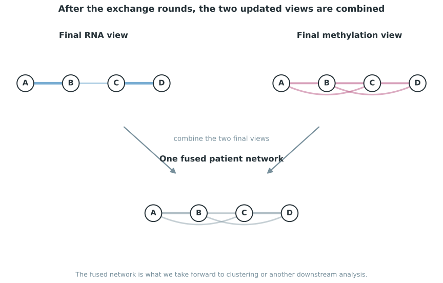
A fused value such as \(P_{fused}(A,B)\) is an integrated network similarity. It describes how strongly the combined evidence from all modalities supports a close connection between A and B. It is not the probability that A and B belong to the same subtype. It is also not a percentage of biological similarity, a gene effect size or a feature loading. A downstream method such as spectral clustering operates on the \(n\times n\) fused network.
The SNF calculation ends with the fused network. Spectral clustering can then be used as a downstream analysis to estimate patient subtypes.
3.11 Four-patient calculation in code
The following code calculates each object separately so that the intermediate matrices can be inspected.
source("scripts/toy-snf-helpers.R")

rna <- rbind(A = c(0, 0), B = c(0.40, 0.10),
             C = c(2.60, 0.10), D = c(3, 0))
meth <- rbind(A = c(0, 0), B = c(1.25, 0.10),
              C = c(1.75, -0.10), D = c(3, 0))

W_rna  <- affinity_from_points(rna,  K = 2, sigma = 0.8)
W_meth <- affinity_from_points(meth, K = 2, sigma = 0.8)

P_rna  <- normalise_P(W_rna)
P_meth <- normalise_P(W_meth)

S_rna  <- trusted_S(P_rna,  K = 2)
S_meth <- trusted_S(P_meth, K = 2)

# One synchronous exchange
new_rna  <- normalise_P(S_rna  %*% P_meth %*% t(S_rna))
new_meth <- normalise_P(S_meth %*% P_rna  %*% t(S_meth))

round(P_rna, 3)
round(S_rna, 3)
round(new_rna, 3)
> round(P_rna, 3)
A B C D
A 0.500 0.394 0.052 0.042
B 0.394 0.500 0.066 0.052
C 0.052 0.066 0.500 0.394
D 0.042 0.052 0.394 0.500
> round(S_rna, 3)
A B C D
A 0.559 0.441 0.000 0.000
B 0.441 0.559 0.000 0.000
C 0.000 0.000 0.559 0.441
D 0.000 0.000 0.441 0.559
> round(new_rna, 3)
A B C D
A 0.500 0.268 0.116 0.108
B 0.268 0.500 0.125 0.116
C 0.116 0.125 0.500 0.268
D 0.108 0.116 0.268 0.500import numpy as np
from scripts.toy_snf_helpers import (
affinity_from_points, normalise_P, trusted_S
)
rna = np.array([[0, 0], [0.40, 0.10], [2.60, 0.10], [3, 0]])
meth = np.array([[0, 0], [1.25, 0.10], [1.75, -0.10], [3, 0]])
W_rna = affinity_from_points(rna, K=2, sigma=0.8)
W_meth = affinity_from_points(meth, K=2, sigma=0.8)
P_rna = normalise_P(W_rna)
P_meth = normalise_P(W_meth)
S_rna = trusted_S(P_rna, K=2)
S_meth = trusted_S(P_meth, K=2)
# One synchronous exchange
new_rna = normalise_P(S_rna @ P_meth @ S_rna.T)
new_meth = normalise_P(S_meth @ P_rna @ S_meth.T)
print(np.round(P_rna, 3))
print(np.round(S_rna, 3))
print(np.round(new_rna, 3))[[0.5 0.394 0.052 0.042]
[0.394 0.5 0.066 0.052]
[0.052 0.066 0.5 0.394]
[0.042 0.052 0.394 0.5 ]]
[[0.559 0.441 0. 0. ]
[0.441 0.559 0. 0. ]
[0. 0. 0.559 0.441]
[0. 0. 0.441 0.559]]
[[0.5 0.268 0.116 0.108]
[0.268 0.5 0.125 0.116]
[0.116 0.125 0.5 0.268]
[0.108 0.116 0.268 0.5 ]]The R and Python helpers agree to three decimal places. This confirms that the row-normalization and neighbour-selection steps perform the same operations in both languages.
3.12 Properties of P and S
3.12.1 Is P a probability?
The rows are normalized in a probability-like way, and a random-walk interpretation is possible. However, SNF should not be interpreted as physically moving a particle between patients. In this chapter, \(P\) is the current normalized sample-similarity network used during diffusion. \(P_{ij}\) is not the probability that two patients belong to the same biological subtype.
3.12.2 Why can a strong edge become smaller?
Normalization redistributes the available weight within each row. When some relationships gain support, others may become smaller. SNF does not make every edge increase in every round.
3.12.3 Is S always symmetric?
No. Local neighbours are selected row by row. Patient A may retain B as one of its strongest neighbours even when B retains a different set. The teaching figures may show an undirected version of the local network, but the row-wise matrix is used in the calculation.
3.12.4 Does S change every round?
No. In the standard SNF algorithm, \(S\) is constructed from the initial normalized network of each modality and remains fixed during diffusion. The matrix \(P\) changes.
3.12.5 Are the original features mixed during diffusion?
No. Once the patient networks have been constructed, diffusion operates on \(n\times n\) patient-similarity matrices. RNA may contain 20,000 genes and methylation may contain 500,000 CpG sites. After conversion, both networks have the same patient-by-patient dimensions.
3.13 Putting the pieces together
The calculation can now be summarized. For each modality, patient distances are converted to the initial affinity matrix \(W\). This matrix is normalized to obtain the evolving matrix \(P\), and its local neighbours are retained in \(S\). During diffusion, each modality updates \(P\) using the other modalities’ previous \(P\) matrices while keeping its own \(S\) fixed. After the selected number of rounds, the final \(P\) matrices are combined into one fused patient network.
This is the same process shown for A, B, C and D in the first chapter. The matrix notation allows it to be applied to hundreds or thousands of patients.