2 DBSCAN in R and Python
2.1 Packages used in this chapter
In R, we will use dbscan (version 1.2.4 at the time of writing), specifically dbscan::dbscan(), dbscan::is.corepoint(), and dbscan::kNNdist(). The package provides a fast implementation of the original algorithm and uses a kd-tree for neighbourhood searches.
In Python, we will use scikit-learn (version 1.9.0), specifically sklearn.cluster.DBSCAN and sklearn.neighbors.NearestNeighbors. The two packages implement the same algorithm from Ester et al. (1996). Near the end of the chapter, we will verify that they produce the same result on our data.
Both packages follow the same convention for minPts / min_samples. The point itself counts as a member of its neighbourhood. Thus MinPts = 4 means four observations in total. That is the point plus three others, not four other observations.
2.2 Loading the data
The eleven labelled points from Chapter 1 are stored in data/dbscan_toy.csv. The larger dataset is in data/dbscan_demo.csv. It was generated with a fixed seed, so R and Python read the same 285 observations.
Keep the downloaded CSV files inside a folder named data when following the examples.
toy <- read.csv("data/dbscan_toy.csv")
print(toy)
id x y
1 A 0.0 0.0
2 B 0.6 0.0
3 C 0.0 0.6
4 D 0.6 0.6
5 E 1.2 0.3
6 F 4.0 0.0
7 G 4.6 0.0
8 H 4.0 0.6
9 I 4.6 0.6
10 J 5.2 0.3
11 K 2.5 3.0import pandas as pd
toy = pd.read_csv("data/dbscan_toy.csv")
print(toy) id x y
0 A 0.0 0.0
1 B 0.6 0.0
2 C 0.0 0.6
3 D 0.6 0.6
4 E 1.2 0.3
5 F 4.0 0.0
6 G 4.6 0.0
7 H 4.0 0.6
8 I 4.6 0.6
9 J 5.2 0.3
10 K 2.5 3.0demo <- read.csv("data/dbscan_demo.csv")
dim(demo)
head(demo, 3)[1] 285 4
id x y true_group
1 1 1.08748638 1.5061594 moon_1
2 2 0.09471056 0.4211638 moon_2
3 3 -1.87250940 1.0616134 moon_1demo = pd.read_csv("data/dbscan_demo.csv")
print(demo.shape)
print(demo.head(3))(285, 4)
id x y true_group
0 1 1.087486 1.506159 moon_1
1 2 0.094711 0.421164 moon_2
2 3 -1.872509 1.061613 moon_1The true_group column is there only so that we can check the result later. It is not passed to DBSCAN. These are the same 285 points shown in Figure 1.1. They form two curved bands surrounded by a loose scatter of observations.
2.3 Fitting the first model
We will begin with \(\varepsilon = 0.3\) and MinPts = 5, the settings used for this dataset in Chapter 1.
library(dbscan)

res <- dbscan::dbscan(as.matrix(demo[, c("x", "y")]), eps = 0.3, minPts = 5)
print(res)
table(res$cluster)
DBSCAN clustering for 285 objects.
Parameters: eps = 0.3, minPts = 5
Using euclidean distances and borderpoints = TRUE
The clustering contains 2 cluster(s) and 17 noise points.
0 1 2
17 134 134
Available fields: cluster, eps, minPts, metric, borderPointsfrom sklearn.cluster import DBSCAN
demo_X = demo[["x", "y"]].to_numpy()
db = DBSCAN(eps=0.3, min_samples=5).fit(demo_X)
print(pd.Series(db.labels_).value_counts().sort_index())-1 17
0 134
1 134
Name: count, dtype: int64The result contains 17 noise points and two clusters of 134 points, corresponding to the two curved bands. eps = 0.3 sets the radius used to search for neighbours. minPts = 5 requires at least five observations, including the point itself, inside that radius before the point is considered core. Later we will use a nearest-neighbour distance plot to see why 0.3 is a reasonable value for eps, and a sensitivity grid to see how much the result depends on both settings.
2.4 Reading the cluster labels
The two outputs use different numbers even though they describe the same clustering. R labels noise as cluster 0 and numbers the clusters 1, 2, .... Scikit-learn labels noise as -1 and numbers the clusters from 0.
This is a bookkeeping difference, not a disagreement about the groups. Apart from the special noise value, the integer assigned to a cluster is arbitrary in both packages. R’s cluster 1, for example, need not represent the same group as Python’s cluster 1. What matters is which observations occur together. When we compare the two implementations later, we will first put their labels onto a common, deterministic scheme.
For plotting, we can translate both conventions into the same readable labels and reuse them throughout the chapter.
canonical_label <- function(cluster, noise_value = 0) {
  ifelse(cluster == noise_value, "Noise", paste("Cluster", cluster))
}
table(canonical_label(res$cluster))
Cluster 1 Cluster 2 Noise
134 134 17def canonical_label(cluster, noise_value=-1):
cluster = pd.Series(cluster)
is_noise = cluster == noise_value
codes = cluster[~is_noise].astype("category").cat.codes + 1
out = cluster.astype(object)
out[~is_noise] = "Cluster " + codes.astype(str)
out[is_noise] = "Noise"
return out
canonical_label(db.labels_).value_counts()Cluster 1 134
Cluster 2 134
Noise 17
Name: count, dtype: int642.5 Identifying core, border, and noise points
Chapter 1 distinguished core, border, and noise points. Both packages give us enough information to recover those categories without reimplementing DBSCAN’s density check.
demo_X <- as.matrix(demo[, c("x", "y")])
core <- dbscan::is.corepoint(demo_X, eps = 0.3, minPts = 5)
kind <- ifelse(res$cluster == 0, "noise", ifelse(core, "core", "border"))
table(kind)
kind
border core noise
18 250 17import numpy as np
core = np.zeros(len(demo_X), dtype=bool)
core[db.core_sample_indices_] = True
noise = db.labels_ == -1
border = (~core) & (~noise)
kind = np.where(noise, "noise", np.where(core, "core", "border"))
pd.Series(kind).value_counts()core 250
border 18
noise 17
Name: count, dtype: int64Both languages find 250 core points, 18 border points, and 17 noise points. In R, is.corepoint() counts each point’s \(\varepsilon\)-neighbourhood and compares that count with minPts. In Python, the fitted object records the core observations in core_sample_indices_. The border points are then the clustered observations left after the core points have been removed. Plotting these three categories gives Figure 1.12 from the previous chapter.
2.6 Checking one neighbourhood by hand
Before relying on the fitted model, let us reproduce its basic calculation for one point. We will inspect the neighbourhood of point D in the toy dataset.
toy_X <- as.matrix(toy[, c("x", "y")])
rownames(toy_X) <- toy$id

d_vec <- toy_X["D", ]
dists_from_D <- sqrt(rowSums((toy_X - matrix(d_vec, nrow(toy_X), 2, byrow = TRUE))^2))
sort(round(dists_from_D, 4))
names(dists_from_D)[dists_from_D <= 0.9]
D B C E A K H F I G J
0.0000 0.6000 0.6000 0.6708 0.8485 3.0610 3.4000 3.4525 4.0000 4.0447 4.6098
[1] "A" "B" "C" "D" "E"import numpy as np
toy_X = toy[["x", "y"]].to_numpy()
d_vec = toy_X[toy["id"].tolist().index("D")]
dists_from_D = np.linalg.norm(toy_X - d_vec, axis=1)
order = np.argsort(dists_from_D)
for i in order:
print(f"{toy['id'][i]}: {dists_from_D[i]:.4f}")
toy["id"][dists_from_D <= 0.9].tolist()D: 0.0000
B: 0.6000
C: 0.6000
E: 0.6708
A: 0.8485
K: 3.0610
H: 3.4000
F: 3.4525
I: 4.0000
G: 4.0447
J: 4.6098
['A', 'B', 'C', 'D', 'E']Five points lie within \(\varepsilon = 0.9\) of D. They are A, B, C, D itself, and E. In the notation of the next chapter, this set is \(N_\varepsilon(D)\). It is the same count illustrated for A in Figure 1.3, now computed directly from the coordinates. We did not call dbscan() here. The calculation shows what the package has to do for every point in the dataset.
2.7 Choosing eps from nearest-neighbour distances
So far we have treated \(\varepsilon\) as given. With a new dataset, a nearest-neighbour distance plot can suggest a useful range to investigate.
The plot turns the core-point definition around. Instead of choosing a radius and counting the points inside it, ask how large the radius around each observation must become before it contains the required number of neighbours. Sorting those radii shows how local density varies across the dataset.
minPts includes the point itself. A distance to the \(k\)-th nearest neighbour, however, normally counts other observations. We therefore use \(k = \text{MinPts} - 1\). With MinPts = 5, the point is the implicit first member of its neighbourhood and the distance of interest is the distance to the fourth other observation.
kdist <- dbscan::kNNdist(demo_X, k = 4)  # k = MinPts - 1 = 5 - 1
kdist_sorted <- sort(kdist)
round(head(kdist_sorted, 5), 4)
round(tail(kdist_sorted, 10), 4)
[1] 0.0810 0.0824 0.0827 0.0827 0.0850
[1] 0.8419 0.8712 1.0677 1.1838 1.3753 1.4061 1.4132 1.4792 1.7381 2.2796from sklearn.neighbors import NearestNeighbors
k = 4 # MinPts - 1 = 5 - 1
nn = NearestNeighbors(n_neighbors=k + 1).fit(demo_X) # +1: the query itself is neighbour 0
dist, _ = nn.kneighbors(demo_X)
kdist_sorted = np.sort(dist[:, k])
print(np.round(kdist_sorted[:5], 4))
print(np.round(kdist_sorted[-10:], 4))[0.081 0.0824 0.0827 0.0827 0.085 ]
[0.8419 0.8712 1.0677 1.1838 1.3753 1.4061 1.4132 1.4792 1.7381 2.2796]The first ten values agree to four decimal places. dbscan::kNNdist(x, k) returns the distance to the k-th nearest other point directly. When scikit-learn queries the training data against itself, the point appears as its own nearest neighbour at distance zero. The Python code therefore requests k + 1 neighbours and takes column k, which is the distance to the k-th other point.
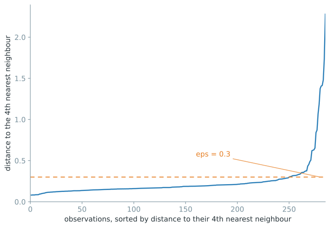
Most observations in demo lie inside one of the dense curved bands and need only a small radius to reach four neighbours. Around rank 260, the curve in Figure 2.1 turns upward. The observations above that bend are comparatively isolated and need a much larger search radius. The line at \(\varepsilon = 0.3\) lies near the bend, making it a sensible candidate to test.
Not every dataset has such a clear knee. Several density levels may produce several bends, while a gradual change in density may produce none. The plot narrows the range worth exploring, but it does not supply a uniquely correct value of \(\varepsilon\).
2.8 Sensitivity to eps
Figure 1.10 showed the visual effect of changing \(\varepsilon\). Here is the corresponding numerical comparison in both languages.
for (eps in c(0.15, 0.3, 0.6)) {
  r <- dbscan::dbscan(demo_X, eps = eps, minPts = 5)
  cat(sprintf("eps=%.2f  clusters=%d  noise=%d\n",
              eps, length(setdiff(unique(r$cluster), 0)), sum(r$cluster == 0)))
}
eps=0.15 clusters=22 noise=133
eps=0.30 clusters=2 noise=17
eps=0.60 clusters=1 noise=10for eps in [0.15, 0.3, 0.6]:
r = DBSCAN(eps=eps, min_samples=5).fit(demo_X)
nc = len(set(r.labels_)) - (1 if -1 in r.labels_ else 0)
print(f"eps={eps:.2f} clusters={nc} noise={(r.labels_ == -1).sum()}")eps=0.15 clusters=22 noise=133
eps=0.30 clusters=2 noise=17
eps=0.60 clusters=1 noise=10The results agree across languages. A small \(\varepsilon\) breaks the data into more than twenty fragments and labels many observations as noise. At 0.3, the two bands are recovered. At 0.6, neighbourhoods span the gap and the bands merge.
2.9 Sensitivity to MinPts
Now hold \(\varepsilon\) at 0.3 and vary the number of observations required for a dense neighbourhood, as in Figure 1.11.
for (mp in c(2, 5, 15)) {
  r <- dbscan::dbscan(demo_X, eps = 0.3, minPts = mp)
  core_r <- dbscan::is.corepoint(demo_X, eps = 0.3, minPts = mp)
  cat(sprintf("MinPts=%2d  core=%3d  clusters=%d  noise=%d\n",
              mp, sum(core_r), length(setdiff(unique(r$cluster), 0)), sum(r$cluster == 0)))
}
MinPts= 2 core=270 clusters=3 noise=15
MinPts= 5 core=250 clusters=2 noise=17
MinPts=15 core= 0 clusters=0 noise=285for mp in [2, 5, 15]:
r = DBSCAN(eps=0.3, min_samples=mp).fit(demo_X)
print(f"min_samples={mp:2d} core={len(r.core_sample_indices_):3d} "
f"clusters={len(set(r.labels_)) - (1 if -1 in r.labels_ else 0)} "
f"noise={(r.labels_ == -1).sum()}")min_samples= 2 core=270 clusters=3 noise=15
min_samples= 5 core=250 clusters=2 noise=17
min_samples=15 core= 0 clusters=0 noise=285With MinPts = 2, a point needs only one other close observation, so 270 of the 285 observations are core. With MinPts = 15, no neighbourhood contains enough observations and the whole dataset is labelled noise. The core count is more informative here than the cluster count. MinPts controls the evidence required to call a neighbourhood dense. Any change in the number of clusters follows from that density decision.
2.10 Why scaling matters
DBSCAN builds its neighbourhoods from distances, so measurement units directly affect the result. The next dataset contains two groups separated only by small_scale_var. The other variable, large_scale_var, has the same distribution in both groups and tells us nothing about group membership, but its values happen to be much larger numerically.
scale_df <- read.csv("data/dbscan_scale_demo.csv")
X_raw <- as.matrix(scale_df[, c("small_scale_var", "large_scale_var")])

r_unscaled <- dbscan::dbscan(X_raw, eps = 15, minPts = 5)
cat("clusters =", length(setdiff(unique(r_unscaled$cluster), 0)),
    " noise =", sum(r_unscaled$cluster == 0), "\n")
table(cluster = r_unscaled$cluster, true_group = scale_df$true_group)
clusters = 1 noise = 2
true_group
cluster 0 1
0 0 2
1 60 58scale_df = pd.read_csv("data/dbscan_scale_demo.csv")
X_raw = scale_df[["small_scale_var", "large_scale_var"]].to_numpy()
r_unscaled = DBSCAN(eps=15, min_samples=5).fit(X_raw)
nc = len(set(r_unscaled.labels_)) - (1 if -1 in r_unscaled.labels_ else 0)
print("clusters =", nc, " noise =", (r_unscaled.labels_ == -1).sum())
pd.crosstab(r_unscaled.labels_, scale_df["true_group"])clusters = 1 noise = 2
true_group 0 1
row_0
-1 0 2
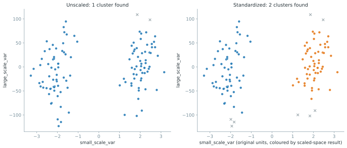
0 60 58Without scaling, DBSCAN places almost all observations in one cluster and labels two as noise. The groups are separated by about 4 units on small_scale_var, whose within-group spread is less than 1. Those differences are overwhelmed by changes of hundreds of units on large_scale_var. Euclidean distance adds squared coordinate differences. It does not know that the larger contribution is irrelevant to the grouping.
X_scaled <- scale(X_raw)  # each column: (x - mean) / sd
round(attr(X_scaled, "scaled:center"), 4)
round(attr(X_scaled, "scaled:scale"), 4)

r_scaled <- dbscan::dbscan(X_scaled, eps = 0.5, minPts = 5)
cat("clusters =", length(setdiff(unique(r_scaled$cluster), 0)),
    " noise =", sum(r_scaled$cluster == 0), "\n")
table(cluster = r_scaled$cluster, true_group = scale_df$true_group)
small_scale_var large_scale_var
-0.024 -3.095
small_scale_var large_scale_var
2.1236 47.8267
clusters = 2 noise = 8
true_group
cluster 0 1
0 3 5
1 57 0
2 0 55col_mean = X_raw.mean(axis=0)
col_std = X_raw.std(axis=0, ddof=1) # ddof=1: same sample-sd convention as R's scale()
X_scaled = (X_raw - col_mean) / col_std
r_scaled = DBSCAN(eps=0.5, min_samples=5).fit(X_scaled)
nc = len(set(r_scaled.labels_)) - (1 if -1 in r_scaled.labels_ else 0)
print("clusters =", nc, " noise =", (r_scaled.labels_ == -1).sum())
pd.crosstab(r_scaled.labels_, scale_df["true_group"])clusters = 2 noise = 8
true_group 0 1
row_0
-1 3 5
0 57 0
1 0 55R’s scale() divides by the sample standard deviation, whose denominator is \(n - 1\). NumPy’s .std() uses the population standard deviation, with denominator \(n\), by default. The Python code passes ddof=1 to match R. Omitting it would produce a plausible result, but the two versions would no longer be carrying out precisely the same transformation.
After standardization, large_scale_var no longer overwhelms small_scale_var. DBSCAN assigns 57 of 60 observations from the first group and 55 of 60 from the second to the corresponding clusters, leaving 8 observations near the boundaries as noise. The before-and-after results appear in Figure 2.2.
Scaling is a modelling decision, not a compulsory preprocessing step. It is appropriate here because the difference in numeric scale comes from the measurement units rather than from meaningful structure. If a variable’s larger range is scientifically important, standardizing it could suppress information that the distance ought to preserve. The choice should follow from what the variables and their units mean.
2.11 Other distance measures
So far we have used Euclidean distance, but DBSCAN is not tied to it. Changing the distance changes which points count as neighbours and can therefore change the clustering, even when \(\varepsilon\) and MinPts stay fixed.
# a precomputed distance object works exactly like the raw feature matrix
d_toy <- dist(toy_X)
res_precomp <- dbscan::dbscan(d_toy, eps = 0.9, minPts = 4)
identical(res_precomp$cluster, dbscan::dbscan(toy_X, eps = 0.9, minPts = 4)$cluster)

# Manhattan distance on the demo data needs a different eps to mean the same thing
res_manhattan <- dbscan::dbscan(dist(demo_X, method = "manhattan"), eps = 0.4, minPts = 5)
cat("Manhattan (eps=0.4): clusters =",
    length(setdiff(unique(res_manhattan$cluster), 0)),
    " noise =", sum(res_manhattan$cluster == 0), "\n")
[1] TRUE
Manhattan (eps=0.4): clusters = 2 noise = 16from scipy.spatial.distance import squareform, pdist
# a precomputed distance matrix works exactly like the raw feature matrix
d_toy = squareform(pdist(toy_X))
res_precomp = DBSCAN(eps=0.9, min_samples=4, metric="precomputed").fit(d_toy)
np.array_equal(res_precomp.labels_, DBSCAN(eps=0.9, min_samples=4).fit(toy_X).labels_)
# Manhattan distance on the demo data needs a different eps to mean the same thing
res_manhattan = DBSCAN(eps=0.4, min_samples=5, metric="manhattan").fit(demo_X)
nc = len(set(res_manhattan.labels_)) - (1 if -1 in res_manhattan.labels_ else 0)
print("Manhattan (eps=0.4): clusters =", nc, " noise =", (res_manhattan.labels_ == -1).sum())True
Manhattan (eps=0.4): clusters = 2 noise = 16Passing a precomputed Euclidean distance matrix through dist() in R or squareform(pdist(...)) in Python reproduces the result obtained from the raw coordinates. Precomputed distances are also useful when similarity is expressed by a domain-specific dissimilarity rather than ordinary coordinates.
The Manhattan example uses eps = 0.4, not 0.3. Manhattan and Euclidean distances have different scales, so a radius chosen for one cannot simply be carried over to the other. There is no claim here that one measure is generally better. The point is that \(\varepsilon\) is measured in the units of the chosen distance, and must be reconsidered whenever that distance changes.
2.12 Why curved clusters work
Neither dbscan() nor DBSCAN() computes a centroid. Each curved band in demo is recovered because its dense neighbourhoods form a connected chain, as described in Chapter 1. The algorithm is not given the shape of either group or the number of groups in advance. The result in Figure 1.12 therefore contains two non-convex clusters that a single centre and radius could not describe.
2.13 Noise does not necessarily mean outlier
The 17 noise points in the main fit are the grey crosses in Figure 1.12. Here, noise means that an observation is not connected to a sufficiently dense region under the chosen \(\varepsilon\) and MinPts.
That label describes density, not data quality. A noise point might be a measurement error, but it might instead be a rare and valid patient profile or a cell between familiar states. Deciding among those interpretations requires subject-matter knowledge. DBSCAN can flag an observation for investigation, but it cannot explain why the observation is unusual.
2.14 Exploring both parameters together
A small grid makes the joint effect of \(\varepsilon\) and MinPts easier to see than changing one value at a time until a preferred cluster count appears.
grid <- expand.grid(eps = c(0.15, 0.2, 0.3, 0.45), minPts = c(3, 5, 10))
grid$clusters <- NA
grid$noise <- NA
for (i in seq_len(nrow(grid))) {
  r <- dbscan::dbscan(demo_X, eps = grid$eps[i], minPts = grid$minPts[i])
  grid$clusters[i] <- length(setdiff(unique(r$cluster), 0))
  grid$noise[i] <- sum(r$cluster == 0)
}
grid
eps minPts clusters noise
1 0.15 3 27 66
2 0.20 3 13 25
3 0.30 3 2 17
4 0.45 3 2 14
5 0.15 5 22 133
6 0.20 5 17 46
7 0.30 5 2 17
8 0.45 5 2 14
9 0.15 10 0 285
10 0.20 10 1 274
11 0.30 10 7 46
12 0.45 10 2 15rows = []
for eps in [0.15, 0.2, 0.3, 0.45]:
for mp in [3, 5, 10]:
r = DBSCAN(eps=eps, min_samples=mp).fit(demo_X)
nc = len(set(r.labels_)) - (1 if -1 in r.labels_ else 0)
rows.append((eps, mp, nc, (r.labels_ == -1).sum()))
pd.DataFrame(rows, columns=["eps", "min_samples", "clusters", "noise"]) eps min_samples clusters noise
0.15 3 27 66
0.15 5 22 133
0.15 10 0 285
0.20 3 13 25
0.20 5 17 46
0.20 10 1 274
0.30 3 2 17
0.30 5 2 17
0.30 10 7 46
0.45 3 2 14
0.45 5 2 14
0.45 10 2 15All twelve combinations give the same cluster and noise counts in R and Python. Several cells contain two clusters, but they do not all represent equally convincing choices. At (eps=0.3, minPts=10), the density requirement is too demanding for the small radius and the bands split into seven pieces. Increasing the radius to 0.45 lets neighbourhoods collect enough points, so (eps=0.45, minPts=10) recovers two clusters. Reading across the grid shows whether a result persists under nearby settings and reveals how one parameter can offset the other.
2.15 Verifying agreement between R and Python
The summaries printed so far agree, but matching totals do not prove that the same observations received the same assignments. We can check the full 285-row result directly.
Because cluster numbers are arbitrary and the packages use different noise values, comparing the raw integers would be meaningless. We first map both results to a deterministic convention. Noise remains a separate category, while the other clusters are sorted by their centroid’s \((x, y)\) position and numbered 1, 2, ... in that order.
def canonical_relabel(df, cluster_col, noise_value):
    is_noise = df[cluster_col] == noise_value
    centroids = df.loc[~is_noise].groupby(cluster_col)[["x", "y"]].mean()
    centroids = centroids.sort_values(["x", "y"])
    remap = {old: new + 1 for new, old in enumerate(centroids.index)}
    out = df[cluster_col].map(remap)
    return out.where(~is_noise, other="noise")
The R and Python results were saved independently and then compared in Python. The comparison produced the following output.
Canonical label agreement: 285 / 285 rows (100.00%)
Mismatched rows: 0
Core-point flag agreement: 285 / 285 rows (100.00%)
Every row has the same canonical cluster or noise label and the same core-point flag. We can also perform a label-independent check by comparing pairs of non-noise observations. For each pair, do both implementations agree that the two observations belong to the same cluster?
Pairwise co-membership check (non-noise pairs in the same cluster):
  pairs flagged same-cluster by R only:      0
  pairs flagged same-cluster by Python only:  0
  pairs both agree are same-cluster:          17822
  agreement rate over the union: 100.00%
The implementations agree on all 17,822 within-cluster pairs, with no one-sided matches. The same check also passes for the eleven-point toy dataset. On both datasets, dbscan::dbscan() and sklearn.cluster.DBSCAN() therefore produce the same partition despite their different label conventions.
2.16 What to carry forward
Every example used the same three ingredients. They were a distance, a radius \(\varepsilon\), and a density threshold MinPts. The dataset, distance measure, and settings changed, but the logic for core, border, and noise points did not. The next chapter develops that logic formally, beginning with a precise definition of what it means for two observations to be close enough.