3 The mathematics behind DBSCAN
3.1 Density and connectivity
Chapter 1 summarized DBSCAN in one sentence.
DBSCAN looks for connected regions built out of locally crowded neighbourhoods.
There are two ideas packed into that sentence. Local crowdedness asks whether enough observations lie near a particular point. Connectivity asks whether nearby crowded regions can be linked into a larger structure. DBSCAN needs both. Density without connectivity would leave us with isolated patches, while connectivity without density could join points through sparse gaps.
We will formalize crowdedness first, then show how DBSCAN connects crowded neighbourhoods into clusters.
3.2 Writing the data mathematically
Collect the observations into a set
\[X = \{x_1, x_2, \ldots, x_n\}.\]
\(X\) denotes the whole dataset, and \(x_i\) denotes its \(i\)th observation, which is one row of the data. If every observation is measured on \(p\) variables, then \(x_i\) is a vector of \(p\) numbers.
\[x_i = (x_{i1}, x_{i2}, \ldots, x_{ip}).\]
For our toy dataset, \(p = 2\) and \(n = 11\). Point \(A\) is
\[x_A = (0, 0),\]
and point \(B\) is
\[x_B = (0.6, 0).\]
The notation is modest but useful. The symbol \(X\) lets us refer to all observations at once, while \(x_i\) lets us discuss any one of them without repeatedly naming its coordinates.
3.3 Measuring closeness
Before we can call a neighbourhood crowded, we need to decide which observations are close. For real-valued coordinates, the most familiar choice is Euclidean distance.
\[d(x_i, x_j) = \sqrt{\sum_{r=1}^{p} (x_{ir} - x_{jr})^2}.\]
In two dimensions, this is the Pythagorean formula. Subtract the first coordinates and square the result, do the same for the second coordinates, add the two squares, and take the square root. The summation sign simply extends that recipe to \(p\) variables.
Check it on \(A\) and \(B\).
\[d(x_A, x_B) = \sqrt{(0 - 0.6)^2 + (0 - 0)^2} = \sqrt{0.36} = 0.6.\]
This agrees with the picture. Points \(A\) and \(B\) are \(0.6\) units apart on the horizontal axis. For a diagonal pair, \(A\) and \(D = (0.6, 0.6)\),
\[d(x_A, x_D) = \sqrt{0.6^2 + 0.6^2} = \sqrt{0.72} \approx 0.849.\]
With \(\varepsilon = 0.9\), \(A\) and \(D\) count as neighbours because \(0.849 < 0.9\), although they are close to the cutoff. Pairs near \(\varepsilon\) are important. A small change in the radius can move them into or out of one another’s neighbourhoods and may alter the resulting clusters.
3.4 Distance to a neighbourhood
A single distance \(d(x_i, x_j)\) tells us about one pair of observations. Crowdedness is different. It asks how many observations surround \(x_i\). We therefore collect every observation within a chosen radius \(\varepsilon\).
\[\boxed{ N_\varepsilon(x_i) = \{\, x_j \in X : d(x_i, x_j) \leq \varepsilon \,\}. }\]
The notation \(N_\varepsilon(x_i)\) means “the \(\varepsilon\)-neighbourhood of \(x_i\).” On the right-hand side, \(x_j \in X\) tells us to consider observations from the dataset. The condition after the colon keeps only those whose distance from \(x_i\) is at most \(\varepsilon\). In plain language, the definition says the following.
Collect every observation that lies no farther than \(\varepsilon\) from \(x_i\).
This is the set represented by the shaded circle in Figure 1.3 from Chapter 1. The picture and the formula describe the same object.
One convention matters throughout the chapter. Since \(d(x_i, x_i) = 0\), every point belongs to its own \(\varepsilon\)-neighbourhood when \(\varepsilon \geq 0\).
\[x_i \in N_\varepsilon(x_i) \quad \text{always.}\]
Thus a neighbourhood count includes the centre point. Remembering this prevents the common off-by-one mistake when interpreting MinPts or computing neighbourhoods by hand.
3.5 Counting nearby observations
Every point has a neighbourhood, whether it lies in a dense region or stands alone. What distinguishes \(A\) from the isolated point \(K\) is the number of observations in that neighbourhood.
We write \(|N_\varepsilon(x_i)|\) for this count. The vertical bars denote the number of elements in the set. Here, that is the number of observations at most \(\varepsilon\) from \(x_i\), including \(x_i\) itself.
For point \(A\) in the toy dataset,
\[N_{0.9}(A) = \{A, B, C, D\},\]
so
\[|N_{0.9}(A)| = 4.\]
Four observations fall within \(0.9\) of \(A\). They are \(A\) itself, plus \(B\), \(C\), and \(D\). We now need to decide how large this count must be before it represents a dense region.
3.6 Setting the density threshold with MinPts
MinPts is the minimum neighbourhood count that DBSCAN will accept as locally dense. What counts as convincing local density depends on the data and the purpose of the analysis.
For the toy dataset, MinPts = 4. Because the centre point is included, this has a concrete interpretation.
MinPts = 4means the point itself, plus at least three other observations, inside its \(\varepsilon\)-neighbourhood.
Both dbscan::dbscan() and sklearn.cluster.DBSCAN() use this convention. Chapter 2’s k-nearest-neighbour distance plot used MinPts = 5 and, correspondingly, \(k = 5 - 1 = 4\) other neighbours.
3.7 Core points can grow a cluster
A point \(x_i\) is a core point when its neighbourhood meets the chosen density threshold.
\[\boxed{ x_i \text{ is a core point} \iff |N_\varepsilon(x_i)| \geq \text{MinPts}. }\]
The symbol \(\iff\) means “if and only if,” or “exactly when.” For \(A\),
\[|N_{0.9}(A)| = 4, \qquad \text{MinPts} = 4, \qquad 4 \geq 4.\]
so \(A\) is core. By contrast, \(E = (1.2, 0.3)\) has
\[N_{0.9}(E) = \{B, D, E\}, \qquad |N_{0.9}(E)| = 3, \qquad 3 \geq 4 \text{ is false.}\]
\(E\) is not core. Its own neighbourhood contains only three points. As we will see shortly, that does not necessarily make \(E\) noise.
3.8 Checking all eleven points
The same calculation can be repeated for all eleven observations. The full pairwise distance matrix is available below for reference. After it, the shorter neighbourhood table records only the distances that pass the \(\varepsilon = 0.9\) cutoff.
| A | B | C | D | E | F | G | H | I | J | K | |
|---|---|---|---|---|---|---|---|---|---|---|---|
| A | 0.000 | 0.600 | 0.600 | 0.849 | 1.237 | 4.000 | 4.600 | 4.045 | 4.639 | 5.209 | 3.905 |
| B | 0.600 | 0.000 | 0.849 | 0.600 | 0.671 | 3.400 | 4.000 | 3.453 | 4.045 | 4.610 | 3.551 |
| C | 0.600 | 0.849 | 0.000 | 0.600 | 1.237 | 4.045 | 4.639 | 4.000 | 4.600 | 5.209 | 3.466 |
| D | 0.849 | 0.600 | 0.600 | 0.000 | 0.671 | 3.453 | 4.045 | 3.400 | 4.000 | 4.610 | 3.061 |
| E | 1.237 | 0.671 | 1.237 | 0.671 | 0.000 | 2.816 | 3.413 | 2.816 | 3.413 | 4.000 | 2.997 |
| F | 4.000 | 3.400 | 4.045 | 3.453 | 2.816 | 0.000 | 0.600 | 0.600 | 0.849 | 1.237 | 3.354 |
| G | 4.600 | 4.000 | 4.639 | 4.045 | 3.413 | 0.600 | 0.000 | 0.849 | 0.600 | 0.671 | 3.662 |
| H | 4.045 | 3.453 | 4.000 | 3.400 | 2.816 | 0.600 | 0.849 | 0.000 | 0.600 | 1.237 | 2.830 |
| I | 4.639 | 4.045 | 4.600 | 4.000 | 3.413 | 0.849 | 0.600 | 0.600 | 0.000 | 0.671 | 3.189 |
| J | 5.209 | 4.610 | 5.209 | 4.610 | 4.000 | 1.237 | 0.671 | 1.237 | 0.671 | 0.000 | 3.818 |
| K | 3.905 | 3.551 | 3.466 | 3.061 | 2.997 | 3.354 | 3.662 | 2.830 | 3.189 | 3.818 | 0.000 |
Computed directly from the coordinates in data/dbscan_toy.csv. See scripts/verify_toy.py.
In each row, retain the entries no larger than \(0.9\). This gives every neighbourhood.
| Point | \(N_\varepsilon(\cdot)\) | \(\lvert N_\varepsilon(\cdot) \rvert\) | Core? |
|---|---|---|---|
| A | \(\{A, B, C, D\}\) | 4 | yes |
| B | \(\{A, B, C, D, E\}\) | 5 | yes |
| C | \(\{A, B, C, D\}\) | 4 | yes |
| D | \(\{A, B, C, D, E\}\) | 5 | yes |
| E | \(\{B, D, E\}\) | 3 | no |
| F | \(\{F, G, H, I\}\) | 4 | yes |
| G | \(\{F, G, H, I, J\}\) | 5 | yes |
| H | \(\{F, G, H, I\}\) | 4 | yes |
| I | \(\{F, G, H, I, J\}\) | 5 | yes |
| J | \(\{G, I, J\}\) | 3 | no |
| K | \(\{K\}\) | 1 | no |
The table identifies eight core points. E and J fall short of the core threshold but sit beside core points, while K has no neighbour other than itself. That distinction leads to the other two point types in DBSCAN.
3.9 Non-core does not mean noise
Consider \(E\) again. It is not core, but declaring it noise immediately would be premature.
Its neighbourhood is \(N_{0.9}(E) = \{B, D, E\}\). Both \(B\) and \(D\) are core points, and \(E\) lies inside both of their neighbourhoods. Although \(E\) cannot support cluster growth on its own, it is directly attached to a dense region. That makes it fundamentally different from \(K\), which lies near no core point. DBSCAN calls a point such as \(E\) a border point.
3.10 Border points belong but cannot grow
A point \(q\) is a border point when two conditions hold. The point \(q\) fails the core test, and it lies within \(\varepsilon\) of at least one core point.
\[\boxed{ q \text{ is a border point} \iff |N_\varepsilon(q)| < \text{MinPts} \ \text{ and there exists a core point } p \text{ with } q \in N_\varepsilon(p). }\]
“There exists” means that at least one suitable core point is enough. The point \(q\) does not have to be near every core point in the dataset.
For \(E\), the first condition holds because \(|N_{0.9}(E)| = 3 < 4\). For the second condition, choose \(p = D\). Point \(D\) is core, and \(E \in N_{0.9}(D) = \{A, B, C, D, E\}\). Therefore \(E\) is a border point. We could equally have used \(p = B\). The same reasoning makes J a border point through either \(G\) or \(I\).
3.11 Noise lies outside every dense region
A point is noise when it is neither core nor border. It is not locally dense itself and does not lie in any core point’s neighbourhood. K is the only such point in the toy dataset. Its neighbourhood count is \(|N_{0.9}(K)| = 1 < 4\), and K appears in none of the core-point neighbourhoods in the table. Under the chosen \(\varepsilon\) and MinPts, it is disconnected from every dense region.
Later, after defining a complete cluster, we will write noise formally as the set of observations left outside all clusters. The two descriptions agree. A non-core point enters a cluster precisely when some core point reaches it as a border point.
3.12 Why one-step definitions are not enough
Core and border points tell us what happens within one neighbourhood, but a cluster may extend through many overlapping neighbourhoods. Suppose \(A\) is core, the core point \(B\) lies in \(A\)’s neighbourhood, another core point lies in \(B\)’s neighbourhood, and the chain continues. Its far end may lie well outside \(A\)’s own \(\varepsilon\)-circle while remaining connected to \(A\) through short local steps.
We therefore need language for one valid step and then for a chain of such steps.
3.13 One step with direct density-reachability
The smallest possible move is one hop from a core point to anything in its neighbourhood. Formally, \(q\) is directly density-reachable from \(p\) when \(q\) lies in \(p\)’s neighbourhood and \(p\) is core.
\[\boxed{ q \text{ is directly density-reachable from } p \iff q \in N_\varepsilon(p) \ \text{ and } \ |N_\varepsilon(p)| \geq \text{MinPts}. }\]
The second condition is simply the core-point test applied to \(p\). In words, the definition says the following.
\(q\) is directly density-reachable from \(p\) exactly when \(q\) lies inside the \(\varepsilon\)-neighbourhood of the core point \(p\).
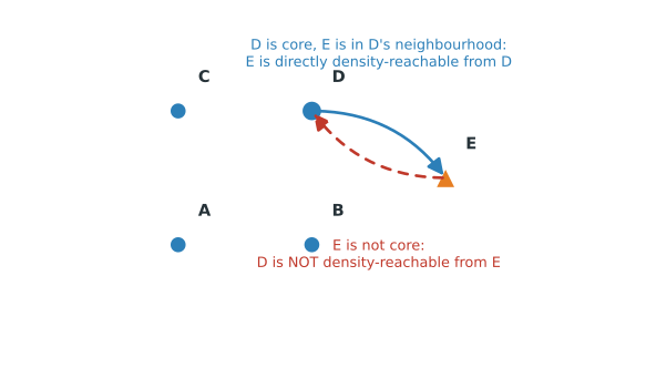
Figure 3.1 shows the idea on the toy dataset. \(D\) is core, and \(E \in N_{0.9}(D)\), so \(E\) is directly density-reachable from \(D\). This formalizes one step of cluster growth. A core point reaches every observation in its neighbourhood.
3.14 Direction matters
The two arrows in Figure 3.1 are deliberately different. The solid arrow from \(D\) to \(E\) is allowed. Reversing it changes which point must pass the core test.
To make \(D\) directly density-reachable from \(E\), we would need both \(D \in N_{0.9}(E)\) and \(E\) to be core. The first condition is true because \(d(D, E) = 0.671 \leq 0.9\), but the second is false because \(|N_{0.9}(E)| = 3 < 4\). Therefore \(D\) is not directly density-reachable from \(E\).
\[q \text{ directly reachable from } p \quad \not\Longrightarrow \quad p \text{ directly reachable from } q.\]
This asymmetry is intentional. The source of a direct reach must be core, whereas the destination need not be. A core point can therefore reach a neighbouring border point, but that border point cannot extend the cluster back out again. This is the mathematical version of the rule from Chapter 1. Border points may join a cluster but may not grow it.
3.15 Many steps with density-reachability
To describe a cluster that extends beyond one neighbourhood, we chain direct reaches together. This requires a sequence of points rather than a single pair.
Let \(p_1, p_2, \ldots, p_m\) be a sequence of observations with \(p_1 = p\) and \(p_m = q\). Say \(q\) is density-reachable from \(p\) when each point in the sequence is directly density-reachable from the one before it.
\[\boxed{ q \text{ is density-reachable from } p \iff \exists\, p_1, \ldots, p_m \text{ with } p_1 = p,\ p_m = q,\ \text{and } p_{r+1} \text{ directly density-reachable from } p_r \text{ for every } r. }\]
Here, “for every \(r\)” means \(r = 1, 2, \ldots, m-1\). Every point \(p_1, \ldots, p_{m-1}\) must be core because it serves as the source of the next hop. The endpoint \(p_m = q\) only needs to be reached, so it may be either core or border. If it is border, the chain ends there.
A one-hop sequence, \(p_1 = p\) and \(p_2 = q\), is direct density-reachability. Longer sequences formalize the linked neighbourhoods shown in Figure 1.6 and Figure 1.9.
3.16 Reachability alone does not mean “same cluster”
Density-reachability remains directional, which makes it unsuitable on its own as a definition of shared cluster membership.
For example, \(E\) is density-reachable from \(A\) through the sequence \(A, D, E\). The first hop is valid because \(A\) is core and \(D \in N_{0.9}(A)\). The second is valid because \(D\) is core and \(E \in N_{0.9}(D)\). In the reverse direction, however, \(E\) cannot supply even the first hop because it is not core. Thus \(A\) is not density-reachable from \(E\).
Yet \(A\) and \(E\) should belong to the same cluster regardless of the order in which we name them. We need a symmetric relation whose truth does not change when the two points are swapped.
3.17 A symmetric relation called density-connectedness
Rather than asking whether one point can reach the other, ask whether a common origin can reach both. Two points \(p\) and \(q\) are density-connected when there is some point \(o\) from which both are density-reachable.
\[\boxed{ p \text{ and } q \text{ are density-connected} \iff \exists\, o \text{ such that } p \text{ is density-reachable from } o \text{ and } q \text{ is density-reachable from } o. }\]
\(o\) is not a centroid or a geometric centre. In the nontrivial cases of interest, it is simply a core point that can grow through the dense structure until it reaches both \(p\) and \(q\).
Figure 3.2 makes this concrete. Take \(o = B\), which is core. Both \(C\) and \(E\) lie in \(N_{0.9}(B)\), so each is directly density-reachable from \(B\) and therefore also density-reachable from it. They are consequently density-connected. This does not require reachability in both directions between \(C\) and \(E\). In fact, \(E\) cannot reach \(C\) because \(E\) is not core.
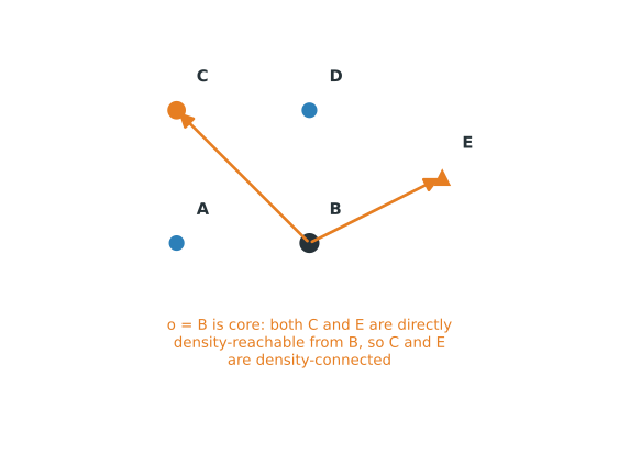
The definition is symmetric by construction. Swapping \(p\) and \(q\) leaves the condition unchanged because both are tested against the same origin \(o\).
3.18 The three relations side by side
The similar names are easier to keep apart when their jobs are compared directly.
| Relation | Question it answers | Core requirement | Symmetric? |
|---|---|---|---|
| Directly density-reachable | Can \(p\) reach \(q\) in one step? | The source \(p\) must be core. The point \(q\) may be core or border. | No |
| Density-reachable | Can \(p\) reach \(q\) through a chain? | The source and every intermediate point must be core. The endpoint \(q\) may be border. | No |
| Density-connected | Can one common origin reach both \(p\) and \(q\)? | For distinct points, the common origin and intermediate points supply the core chain. Either endpoint may be border. | Yes |
The progression is one step, then many steps, then a shared origin. The first two relations describe how a cluster can grow. The third lets us state that two observations belong to the same dense, connected structure without choosing one of them as the starting point.
3.19 Defining a DBSCAN cluster
A cluster \(C\) is a subset of \(X\) satisfying two conditions.
Connectivity. Any two observations in \(C\) are density-connected.
\[\forall\, p, q \in C: \ p \text{ and } q \text{ are density-connected.}\]
Maximality. If \(p \in C\) and some point \(q \in X\) is density-reachable from \(p\), then \(q \in C\) as well. In other words, the cluster may not stop partway through a valid chain of reachability.
\[\forall\, p \in C,\ q \in X: \quad q \text{ density-reachable from } p \implies q \in C.\]
\[\boxed{ \text{A DBSCAN cluster } C \text{ is a maximal, density-connected subset of } X. }\]
“Maximal” does not mean “largest cluster in the dataset.” It means that the set already contains every point reachable from any of its members. We cannot add another reachable point while preserving the definition. Connectivity keeps the set in one piece, and maximality prevents us from stopping early. This is why E and J are included as endpoints of valid chains and why the cluster boundary appears where its core-point chain runs out, as in Figure 1.12.
3.20 Formal definition of noise
Suppose DBSCAN discovers clusters \(C_1, C_2, \ldots, C_K\). Noise is the set of observations that belong to none of them.
\[\boxed{ \text{Noise} = X \setminus \bigcup_{k=1}^{K} C_k. }\]
The symbol \(\bigcup_{k=1}^{K} C_k\) means the union of all clusters. It includes every observation belonging to at least one \(C_k\). The symbol \(\setminus\) means set subtraction. Thus the formula says the following.
Start with every observation in the dataset. Remove every observation that belongs to some cluster. Whatever is left over is noise.
For the toy dataset, \(C_1 = \{A, B, C, D, E\}\) and \(C_2 = \{F, G, H, I, J\}\). Their union contains ten of the eleven points, so subtracting it from \(X\) leaves \(\{K\}\).
3.21 The same idea as a graph
The definitions above can also be expressed as a graph. This view often makes the role of the core points easier to see.
Take only the core points and build a graph on them. Draw an edge between two core points whenever their distance is at most \(\varepsilon\). Call this the core graph.
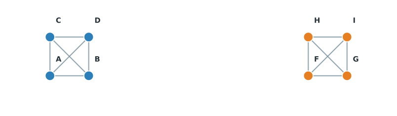
Figure 3.3 shows the result for the toy dataset. It has two connected components, \(\{A, B, C, D\}\) and \(\{F, G, H, I\}\), because every distance between the two groups exceeds \(\varepsilon\). A connected component is a maximal group of nodes linked by paths. Any node in the component can be reached from any other by following edges, and no node outside the component is reachable in this way.
These components are the cluster backbones from Chapter 1.
\[\boxed{ \text{connected components of the core graph} = \text{cluster backbones.} }\]
To obtain the full clusters, attach a non-core point when it lies in the \(\varepsilon\)-neighbourhood of a core point in the component.
\[\boxed{ \text{DBSCAN cluster} = \text{connected core component} + \text{adjacent border points.} }\]
For core points, density-reachability has become an ordinary graph question. Do the two nodes belong to the same connected component? Border points are then attached at the boundary. If a border point touches core points in two different components, it is eligible for either cluster. The implementation must choose one. We return to that special case in the section on border-point ambiguity.
3.22 Local steps can produce large clusters
The graph view also explains how two observations much farther than \(\varepsilon\) apart can belong to one cluster.
Suppose \(q\) is density-reachable from \(p\) through a chain \(p_1, p_2, \ldots, p_m\) with \(p_1 = p\) and \(p_m = q\). The definition only constrains consecutive points in the chain.
\[d(p_r, p_{r+1}) \leq \varepsilon \quad \text{for every } r.\]
There is no requirement that the two endpoints themselves be neighbours. The triangle inequality gives
\[d(p_1, p_m) \leq \sum_{r=1}^{m-1} d(p_r, p_{r+1}) \leq (m-1)\varepsilon,\]
so the possible endpoint distance grows with the number of hops rather than being capped at \(\varepsilon\).
For a concrete one-dimensional example, place nine observations at
\[0,\ 0.6,\ 1.2,\ \ldots,\ 4.8\]
and use \(\varepsilon = 0.7\) with MinPts = 3. Each interior point sees itself and its two immediate neighbours, so it is core. The two endpoints are border points reached by the neighbouring core points. All nine observations therefore form one cluster, even though its diameter is \(4.8\), almost seven times \(\varepsilon\). Figure 1.9 illustrates the same principle in a curved geometry. Local links, rather than endpoint distance, hold the cluster together.
3.23 Turning the definitions into an algorithm
The algorithm follows the definitions closely. It keeps two pieces of information separate.
- whether a point has been visited, meaning its neighbourhood has been examined
- its current label, which may be unassigned, noise, or a cluster identifier
When DBSCAN visits a point, it computes the point’s \(\varepsilon\)-neighbourhood. A non-core point is provisionally labelled noise unless an expanding cluster has already claimed it. An unassigned core point starts a new cluster. The algorithm then works through its neighbours. Each core neighbour contributes its own neighbourhood to the search, so the cluster continues growing. A non-core neighbour joins as a border point but contributes nothing further. Expansion stops when there are no new reachable points to process, matching the behaviour in Figure 1.7.
for each point p in X:
    if visited(p):
        continue
    visited(p) = true
    N = neighbourhood(p, eps)
    if |N| < MinPts:
        label(p) = NOISE        # provisional, may still become a border point
        continue

    start a new cluster C
    add p to C
    seeds = N \ {p}
    while seeds is not empty:
        q = remove one point from seeds
        if not visited(q):
            visited(q) = true
            Nq = neighbourhood(q, eps)
            if |Nq| >= MinPts:  # q is core: it can extend the search further
                seeds = seeds union Nq
        if label(q) is UNASSIGNED or NOISE:
            label(q) = C        # add q as core or border, replacing provisional noise
A point can be marked NOISE early because the core point that will eventually reach it has not yet been processed. If a later expansion reaches that point, its label changes from NOISE to the current cluster. Its neighbourhood does not need to be recomputed. The value of visited(q) records that it was already checked and found non-core. Thus “labelled noise at this moment” is not the same as noise in the final clustering.
3.24 Running the toy dataset by hand
We can now reproduce DBSCAN’s output for all eleven points from the neighbourhood table alone. Visit the points in alphabetical order.
Visit A. Point \(A\) is unvisited. Its neighbourhood is \(N_{0.9}(A) = \{A, B, C, D\}\), which has size 4, so it is core. Start Cluster 1 and add \(A\). The seeds are \(\{B, C, D\}\).
Expand seed B. Point \(B\) is unlabelled, so add it to Cluster 1. Its neighbourhood is \(N_{0.9}(B) = \{A, B, C, D, E\}\), which has size 5, so it is core. Add its neighbourhood to the seed queue. This introduces \(E\) as a new seed.
Expand seed C. Point \(C\) is unlabelled, so add it to Cluster 1. Its neighbourhood is \(N_{0.9}(C) = \{A, B, C, D\}\), which has size 4, so it is core. Every member is already in Cluster 1 or already queued, so there are no new seeds.
Expand seed D. Point \(D\) is unlabelled, so add it to Cluster 1. Its neighbourhood is \(N_{0.9}(D) = \{A, B, C, D, E\}\), which has size 5, so it is core. Point \(E\) is already queued, so there is still no new seed beyond it.
Expand seed E. Point \(E\) is unlabelled, so add it to Cluster 1. Its neighbourhood is \(N_{0.9}(E) = \{B, D, E\}\), which has size 3. It is not core, so its neighbourhood is not added to the queue. Point \(E\) ends this branch as a border point.
The seeds are exhausted. Cluster 1 is finished and contains \(\{A, B, C, D, E\}\).
Visit F. Point F is unvisited because it does not appear in any neighbourhood expanded for Cluster 1. Its neighbourhood is \(N_{0.9}(F) = \{F, G, H, I\}\), which has size 4, so it is core. Start Cluster 2. The same expansion plays out on the second backbone. Points \(G\) and \(I\) are added and are core, with each one reaching \(J\). Point \(H\) is also core but contributes nothing new. Point \(J\) is processed last and has \(N_{0.9}(J) = \{G, I, J\}\) of size 3, so it is not core. It ends that branch as a border point.
Cluster 2 is finished and contains \(\{F, G, H, I, J\}\).
Visit K. Point \(K\) is unvisited. Its neighbourhood is \(N_{0.9}(K) = \{K\}\), which has size 1, so it is not core. Point \(K\) is provisionally labelled noise. No cluster ever reaches it. It does not appear in any core point’s neighbourhood anywhere in the distance table above. Its provisional label never changes.
Every point has now been visited. The result is shown below.
\[C_1 = \{A, B, C, D, E\}, \qquad C_2 = \{F, G, H, I, J\}, \qquad \text{Noise} = \{K\}.\]
This matches Chapters 1 and 2. Points A, B, C, D, F, G, H, I are core, E and J are border, and K is noise. The package implementations automate the same neighbourhood checks carried out here by hand.
3.25 How \(\varepsilon\) changes density
Return to the core-point condition, \(|N_\varepsilon(x_i)| \geq \text{MinPts}\). Increasing \(\varepsilon\) makes the condition \(d(x_i, x_j) \leq \varepsilon\) easier to satisfy, so a neighbourhood can gain members but cannot lose them.
\[\varepsilon_1 < \varepsilon_2 \implies N_{\varepsilon_1}(x_i) \subseteq N_{\varepsilon_2}(x_i) \implies |N_{\varepsilon_1}(x_i)| \leq |N_{\varepsilon_2}(x_i)|.\]
With MinPts fixed, increasing \(\varepsilon\) can therefore turn a non-core point into a core point, but never the reverse. Existing reachability links also remain, while new ones may appear. Consequently, clusters may expand or merge and noise may become part of a cluster. This behaviour follows directly from the nested-neighbourhood relation above. Figure 1.10 is a visual example of it.
3.26 How MinPts changes density
Now hold \(\varepsilon\), and therefore every neighbourhood, fixed. Raising MinPts raises the threshold that each neighbourhood count must clear. A point that is core at MinPts = 4 may fail the test at MinPts = 15 even though none of its distances has changed. Chapter 2’s demo showed exactly this. With the same 285 observations and \(\varepsilon = 0.3\), increasing MinPts from 5 to 15 reduced the number of core points from 250 to zero. Only the threshold changed.
3.27 One density rule
The two parameters act on opposite sides of one comparison. A larger \(\varepsilon\) tends to collect more observations into each neighbourhood. A larger MinPts demands a larger count before accepting that neighbourhood as dense.
\[|N_\varepsilon(x_i)| \geq \text{MinPts}.\]
The table reuses the core-point counts from Chapter 2’s 285-observation demo.
| Setting | eps | MinPts | Core points |
|---|---|---|---|
| baseline | 0.30 | 5 | 250 |
| larger eps, same MinPts | 0.45 | 5 | 268 |
| same eps, larger MinPts | 0.30 | 15 | 0 |
Increasing \(\varepsilon\) can raise the left-hand side, while increasing MinPts raises the right-hand side. If both increase, their effects may partly offset one another. It is therefore more useful to think of them as a pair that defines one notion of density than as unrelated settings tuned in isolation.
3.28 Deriving the k-distance plot
The k-distance plot from Chapter 2 follows directly from the core-point condition. Fix MinPts = m. Because \(x_i\) counts itself, \(x_i\) is core when at least \(m - 1\) other observations lie within \(\varepsilon\).
For each observation \(x_i\), define \(r_k(x_i)\) as the distance from \(x_i\) to its \(k\)-th nearest other observation, with
\[k = m - 1.\]
Then
\[r_k(x_i) \leq \varepsilon \quad \Longleftrightarrow \quad |N_\varepsilon(x_i)| \geq m.\]
The left side says that the \(k\)th other neighbour is within the radius. The right side says that the neighbourhood contains at least those \(k\) observations plus \(x_i\) itself. Extra observations and distance ties do not cause a problem because the requirement is at least \(m\), not exactly \(m\).
Compute \(r_k(x_i)\) for every observation and sort the values. This produces Figure 2.1 from Chapter 2. Points in dense regions need only a small radius to collect \(k\) neighbours and appear near the low end of the curve. Points in sparse regions need a larger radius and appear near the high end. A pronounced rise suggests a transition between the two regimes and gives a plausible range for \(\varepsilon\).
The derivation does not guarantee a single, unambiguous bend. Data with several density levels may produce several bends, and gradual changes in density may produce no sharp bend at all. The plot is a diagnostic, not a formula that returns one correct value.
3.29 Scale is part of the distance
For two variables, Euclidean distance is
\[d(x_i, x_j) = \sqrt{(x_{i1} - x_{j1})^2 + (x_{i2} - x_{j2})^2}.\]
Suppose two observations differ by \(0.5\) in the first variable and by \(500\) in the second. Then
\[d = \sqrt{0.5^2 + 500^2} = \sqrt{0.25 + 250000} = \sqrt{250000.25} \approx 500.0003.\]
The second variable contributes \(250000\) inside the square root, while the first contributes only \(0.25\). For practical purposes, \(d \approx 500\). The first variable has almost no influence on the result. In Chapter 2’s scaling example, large_scale_var varied across hundreds of units despite carrying no information about the true groups. Without scaling, it overwhelmed small_scale_var, the informative variable, and DBSCAN placed 118 of the 120 observations in one cluster, leaving two as noise.
Standardizing removes this asymmetry directly. For variable \(j\), replace each raw value with
\[z_{ij} = \frac{x_{ij} - \bar{x}_j}{s_j}.\]
This subtracts the column mean \(\bar{x}_j\) and divides by its standard deviation \(s_j\). For any non-constant variable, the standardized values have mean \(0\) and standard deviation \(1\). A difference of one standardized unit therefore represents one standard deviation, regardless of the original units.
3.30 What changes in high dimensions
DBSCAN relies on distance to distinguish a crowded neighbourhood from the space around it. As the number of variables grows, that distinction can become less pronounced, especially when many variables contribute independent variation but little useful structure.
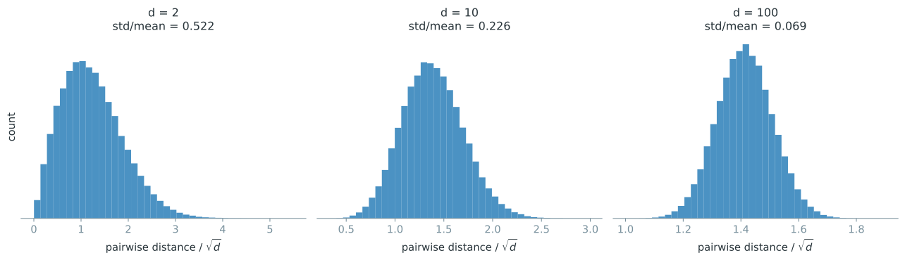
Figure 3.4 isolates this effect with 600 random points whose coordinates are independent standard-normal values. It shows \(d = 2\), \(d = 10\), and \(d = 100\), with pairwise distances divided by \(\sqrt{d}\) so that the panels fit on comparable axes. The standard deviation of the distances, relative to their mean, falls from \(0.52\) in two dimensions to \(0.23\) in ten and \(0.07\) in one hundred. In this unstructured example, pairwise distances become increasingly similar relative to their typical size. The contrast between “near” and “far” is much weaker in the final panel.
For DBSCAN, weaker distance contrast makes a useful \(\varepsilon\) harder to find. A small change in the radius may move many observations into or out of a neighbourhood at once, and the k-distance curve may offer no clear knee. Irrelevant variables can make this worse by adding differences that have nothing to do with the groups of interest. Depending on the radius, the result may then swing between many noise points and large, merged clusters.
The figure does not show that every high-dimensional dataset lacks meaningful neighbours. Real data may contain strong separation, lie near a lower-dimensional structure, or use a domain-specific distance that preserves useful similarity. The practical lesson is narrower. Thousands of raw features should not be handed to a distance-based method without examining what those features make “close” mean. Feature selection, a defensible dimensionality reduction, or a distance chosen for the scientific setting may help. None is an automatic fix, and PCA is not automatically the right choice.
3.31 When a border point touches two clusters
A border point’s cluster assignment is not always unique. This follows from the definition rather than from an error in a particular implementation.
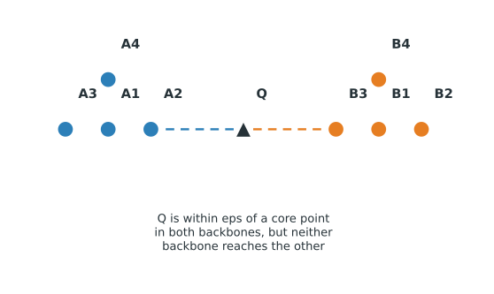
In Figure 3.5, the blue and orange core points form separate components. No core point in one component lies within \(\varepsilon\) of a core point in the other. Point \(Q\), however, is within \(\varepsilon\) of a core point on each side. It satisfies the border-point definition for both components. The definition itself gives no reason to prefer one.
The original DBSCAN procedure assigns \(Q\) to whichever cluster reaches it first. Changing the visit order can therefore change \(Q\)’s label. This ambiguity is limited to contested border points. It cannot move a core point from one core component to another or merge the two backbones. There is no general promise that only a small number of points will be contested, although in many datasets the issue affects only observations near a boundary.