1  DBSCAN

1.1 Two curves, no labels

Here are 260 points measured on two variables, together with a handful of scattered ones.

Figure 1.1: 260 observations forming two curved bands, plus a scattering of isolated points.

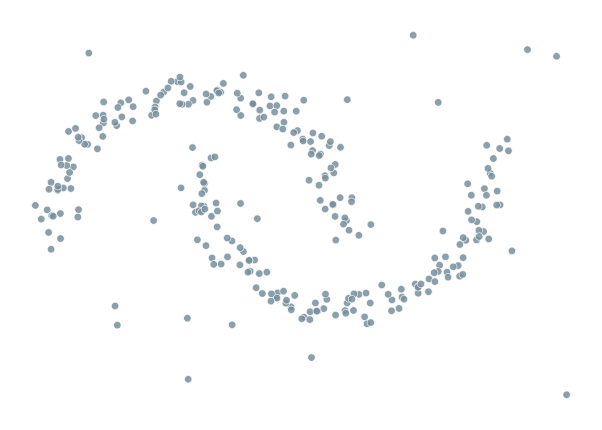
Spend a few seconds with Figure 1.1 before reading on. Most people see two curved bands and a loose scatter of points that do not belong to either one. Yet there is no legend, colour, or label telling you where the groups are. What in the picture creates that impression?

Put the impression into words and it comes down to something simple. Inside each band, points sit close together, while the points outside are spread thin and mostly alone. DBSCAN is built around that contrast between crowded and sparse regions. The rest of the chapter turns it into a rule a computer can follow.

1.2 Why centres miss the shape

A familiar way to describe a group of points is to give it a centre, then assign nearby points to that centre. That is the approach used by k-means, and it works well for compact, roughly round groups. These bands are a different shape.

Figure 1.2: Splitting the two bands by distance to two centroids cuts straight across both of them, compared with the curved groups a person would actually draw.

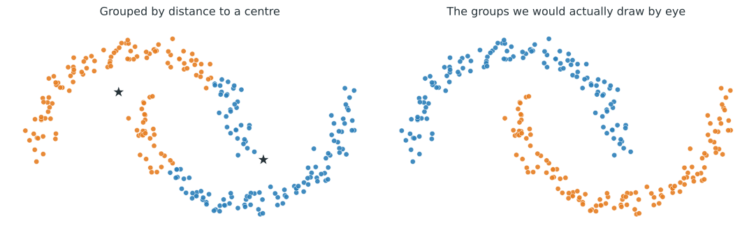
In the left panel of Figure 1.2, each point is assigned to the nearer of the two centroids, shown as black stars. The resulting boundary cuts straight through both curved bands. The right panel shows the grouping most people would draw by eye. Neither band has one useful centre for all of its points. Because the bands are long and curved, a point near one end can be closer to the other band’s centre than to its own.

This does not mean k-means has failed. It is answering the question it was designed to answer. “Which centre is this point nearest to?” DBSCAN asks a different question. “Which crowded region is this point part of?” It answers by looking at the area immediately around each point rather than measuring everything against a global centre.

1.3 Crowded meaning

Choose one point and ask whether it sits somewhere crowded. A natural test is to look a fixed distance around it and count the observations that fall inside.

Figure 1.3: One point, drawn in black, with every observation inside a fixed radius of it drawn in blue.

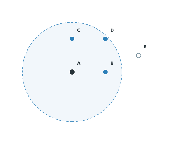
Figure 1.3 draws that circle around point A. Three other points, B, C, and D, fall inside it. E does not. The contents of this circle give us the local information we need to judge how crowded A’s surroundings are.

DBSCAN calls the fixed radius eps, usually written with the Greek letter \(\varepsilon\). For the rest of this course, we use a small labelled dataset of eleven points, A through K, with \(\varepsilon = 0.9\). We will use these same points again in the practice and mathematics chapters.

1.4 A radius still needs a head count

The radius tells us where to look, but not how many observations make the area dense. Two points can happen to sit close together in an otherwise empty stretch of the data. That pair alone should not automatically become a cluster.

Figure 1.4: The same radius drawn around two different points. One circle contains five observations. The other contains only the point itself.

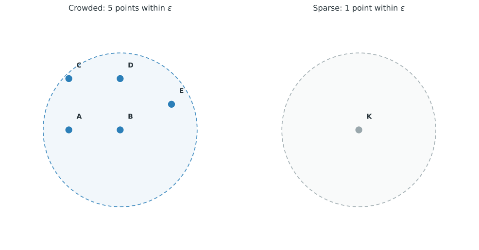
Both circles in Figure 1.4 have radius \(\varepsilon = 0.9\). The circle centred on B contains five observations, while the one centred on K contains only K. The scale is the same, but the local head count is not.

DBSCAN therefore needs a second setting. It is the minimum number of observations a neighbourhood must contain before it counts as dense. This threshold is called MinPts. We will use MinPts = 4, so B’s neighbourhood easily qualifies and K’s does not. Remember that the centre point counts too. Its distance from itself is zero, which always places it inside its own neighbourhood.

1.5 Core points can lead

Those two settings are enough to define the first of DBSCAN’s three kinds of point.

Figure 1.5: Three focused views of a core point, a border point, and a noise point in the toy dataset. Each view includes its own epsilon circle.

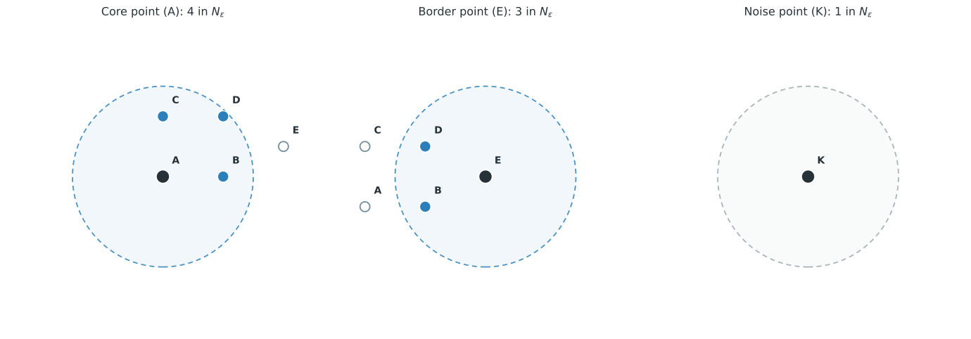
The left panel of Figure 1.5 shows A again. Its \(\varepsilon\)-neighbourhood contains four observations, including itself. They are A, B, C, and D. With MinPts = 4, it meets the threshold exactly. A core point is any point whose neighbourhood contains at least MinPts observations. In this dataset, A, B, C, and D are all core, as are F, G, H, and I on the other side. Together, they mark the locally dense parts of the dataset.

1.6 Border points are close enough to belong

Now look at point E in the middle panel. Its neighbourhood contains only three observations. They are B, D, and E itself. It falls one short of MinPts = 4, so E is not core.

Throwing E away would still feel wrong. It lies inside D’s neighbourhood, and D is core. In other words, E is not in a dense enough position to qualify by itself, but it is right beside a region that does qualify.

A border point is a non-core point that falls inside the \(\varepsilon\)-neighbourhood of at least one core point. E qualifies because it lies within reach of D. It belongs to the cluster, but it cannot extend the cluster. The difference between belonging and providing the density needed for further growth is central to how DBSCAN works.

1.7 Noise is a label, not a verdict

The right panel of Figure 1.5 shows K. Its neighbourhood contains only itself, so it is not core. Unlike E, it also lies outside every core point’s neighbourhood.

A point that is neither core nor a border point is called noise. The term can sound stronger than it is. Calling K noise does not mean it is a measurement error or a bad observation. It means only that, for the chosen \(\varepsilon\) and MinPts, K is not connected to a sufficiently dense region. With different settings, it might join a cluster, while a point currently in a cluster might become noise. The label depends on the density threshold. It is not a permanent fact about the observation.

1.8 Building the dense backbone

One core point accounts for only a small circle. A cluster can grow much larger by linking one core point to another.

Figure 1.6: Four steps of the same cluster growing, one core point at a time, as overlapping epsilon neighbourhoods are added.

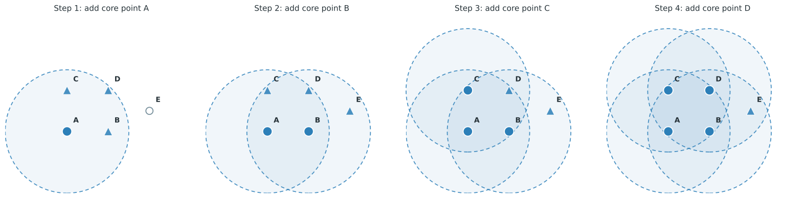
Step 1 of Figure 1.6 begins at A. Because A is core, its whole neighbourhood, {A, B, C, D}, enters the cluster. B, C, and D are included immediately because they lie inside A’s circle.

Step 2 checks B. Since B is also core, its neighbourhood is added as well. The cluster is no longer limited to the circle around A. Whenever a newly reached point is core, its own neighbourhood can carry the cluster farther. Steps 3 and 4 do the same for C and D, leaving four overlapping circles and one continuous dense region.

Together, these core points form the cluster’s backbone. Each contributes a dense neighbourhood, and the overlaps allow the backbone to spread. A border point is included when the search reaches it, but its neighbourhood does not drive further expansion. It ends the chain instead of extending it.

1.9 Border points stop the chain

The example below shows why DBSCAN expands through core points only.

Figure 1.7: A core point reaches a border point, but a further point beyond the border point cannot join, because the border point is not itself core.

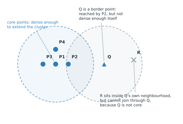
In Figure 1.7, four core points form a small dense backbone. Q lies inside the neighbourhood of the rightmost core point, so it joins the cluster as a border point. R, farther to the right, lies inside Q’s neighbourhood. If Q were allowed to expand the cluster as a core point does, R would be pulled in next.

But Q is not core. Its neighbourhood contains only two other observations, or three once Q itself is counted, so it does not meet MinPts = 4. Allowing every nearby point to continue the search would let one stray observation at the edge of a cluster pull in a whole trail of loosely scattered points. Restricting expansion to core points makes the search stop when the data becomes sparse. Since R can be reached only through non-core Q, it stays outside the cluster.

1.10 A thin bridge does not join two clusters

The same rule prevents two dense groups from merging merely because a few scattered points lie between them.

Figure 1.8: A dense group of points on the left and another on the right, connected only by a thin, evenly spaced chain of isolated points, none of which is core.

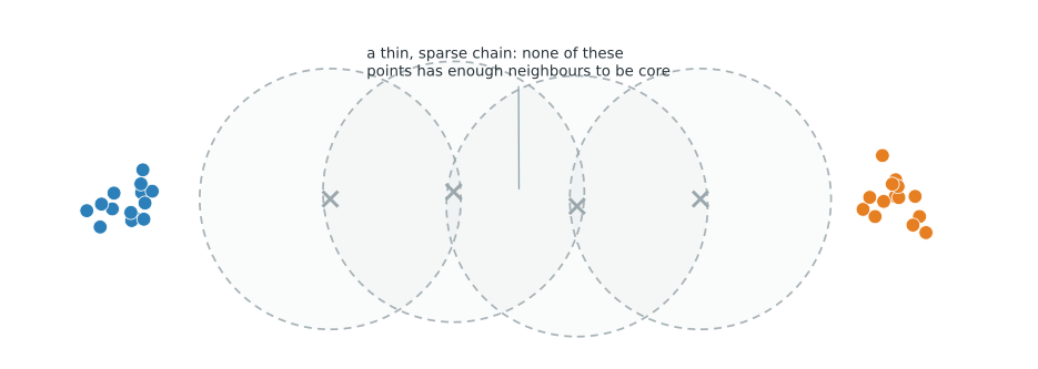
Figure 1.8 shows two dense groups connected by a thin trail of four points. If any pair of points within \(\varepsilon\) could extend a cluster, the trail would stitch the groups together. Each bridge point is close enough to the next one.

Now count each bridge point’s neighbourhood. At most, it contains the point itself and its two immediate neighbours. That gives three observations, one short of the four required by MinPts. None of the bridge points is core, so none can carry a cluster across the gap. DBSCAN leaves the dense groups as separate clusters and labels the four points between them as noise.

1.11 Following a cluster to its edge

DBSCAN picks an unvisited point and checks its neighbourhood. If the point is core, a new cluster starts there. Its neighbours are added. Any of those that are also core contribute their own neighbours. The search continues until no new core point remains to expand. The border points stay attached at the edge. DBSCAN then moves to another unvisited point and looks for the start of the next cluster.

On the eleven-point dataset, this happens in two passes. Starting from A, DBSCAN builds the backbone {A, B, C, D} and attaches E as a border point. Once there are no more core points to follow, the first cluster is complete. Later, the search reaches unvisited core point F. The set {F, G, H, I} becomes the second backbone, with J on its border. K never becomes core and never falls inside a core point’s neighbourhood, so it finishes as noise.

There is one wrinkle in that description. A point may be marked as noise when it is first checked, then later be reached by a core point and relabelled as a border point. Its final status is not necessarily settled on the first visit. It is settled by the completed search.

1.12 A cluster can be much wider than \(\varepsilon\)

Chaining through core points has a consequence that is easy to miss. Two points in the same DBSCAN cluster need not be close to each other.

Figure 1.9: Two points at opposite ends of the same curved cluster, with an orange route following the band and a dashed line showing the direct distance between them.

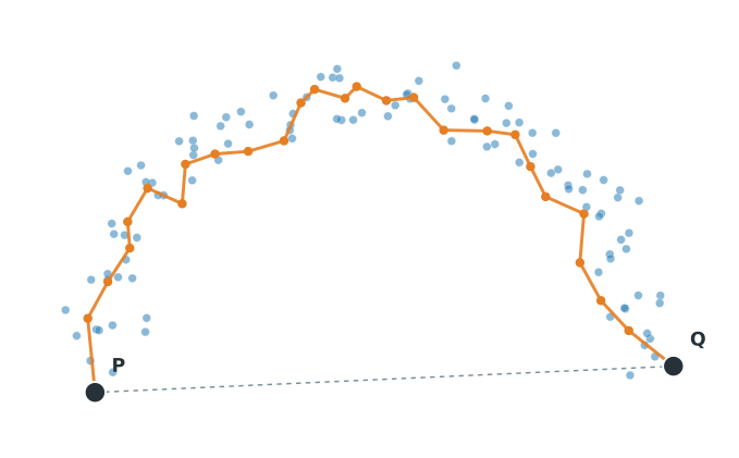
P and Q in Figure 1.9 sit at opposite ends of the same curved band. Their straight-line distance, shown by the dashed line, is much larger than \(\varepsilon\). The orange line is a visual guide along the band, passing through nearby observations rather than cutting across the empty space. It is not the exact neighbourhood-by-neighbourhood route taken by DBSCAN, so its individual drawn segments should not be read as guaranteed \(\varepsilon\)-sized hops.

The actual DBSCAN connection comes from a chain of overlapping core neighbourhoods spanning the band, with P or Q attaching at the ends if either happens to be a border point. That chain may use more intermediate points than the orange guide shows. What matters is local density along the band. The two ends never need to be near each other. In other words, \(\varepsilon\) limits the size of an individual neighbourhood, not the width or diameter of a whole cluster. A cluster can span many times \(\varepsilon\) as long as a continuous dense path holds it together.

1.13 Turning eps down and up

So far, both settings have stayed fixed. Figure 1.10 shows what changes when only \(\varepsilon\) moves.

Figure 1.10: The same 285 observations clustered with three different values of eps while MinPts stays fixed. The values range from too small, through a sensible choice, to too large.

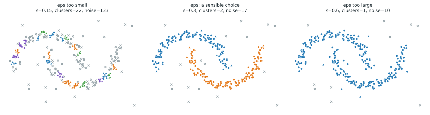
In the left panel, \(\varepsilon\) is too small. Few neighbourhoods collect MinPts observations, so the bands break into more than twenty small fragments and much of the data is labelled noise. The reason is direct. A smaller radius captures fewer observations, leaving fewer points able to qualify as core.

The middle panel uses a more suitable radius. Each curved band becomes one coherent cluster, while the scattered background points remain noise. In the right panel, \(\varepsilon\) is large enough for points between the bands to connect dense neighbourhoods on both sides. What looked like two clusters is now merged into one. The data is identical in all three panels. Only the radius changes.

1.14 Raising and lowering the MinPts bar

This time, keep \(\varepsilon\) fixed and change the amount of local evidence required for density.

Figure 1.11: The same dataset clustered with three different values of MinPts while eps stays fixed. The values range from too small, through a sensible choice, to too large.

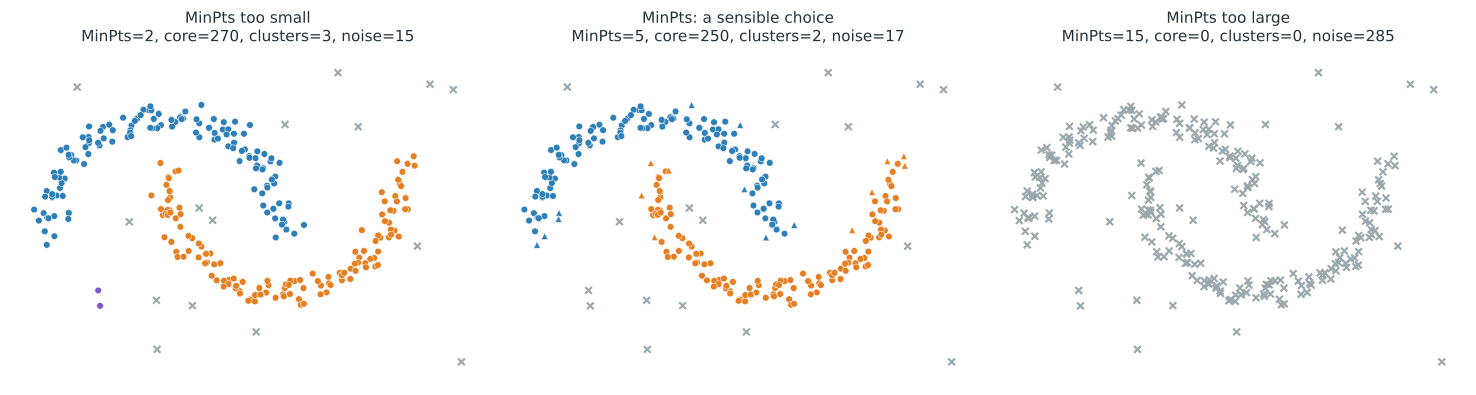
In the left panel of Figure 1.11, MinPts = 2, so an observation needs only one other nearby point to qualify as core. Here, 270 of the 285 points do so, which means the density requirement is barely filtering anything. The middle panel asks for more neighbours. A ring of border points appears around a smaller core, making the core-and-border structure easier to see in this larger dataset.

In the right panel, MinPts is higher than any neighbourhood count in the dataset. No point clears the bar, so every point becomes noise. It is tempting to reduce this to “larger MinPts means fewer clusters,” but cluster counts do not change that neatly. A better interpretation is that MinPts controls how much nearby support a point needs before DBSCAN treats its location as dense. Raising that demand can shrink the cores, create more noise, or break a previously connected cluster into pieces.

1.15 Reading the final result

With a suitable \(\varepsilon\) and MinPts, the full dataset produces the result below.

Figure 1.12: The final DBSCAN result contains two clusters, each with a solid core backbone and a ring of attached border points, plus scattered noise.

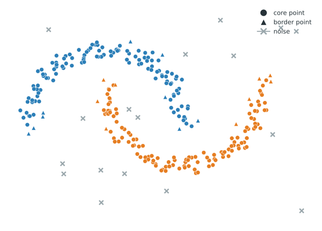
Every marker in Figure 1.12 has one of the three roles introduced in this chapter. Circles mark core points and form the dense backbone of each band. Triangles mark border points along the thinner edges. Grey crosses mark noise, meaning observations that never connect to either backbone. We did not choose the number of clusters in advance, and DBSCAN never computed a centroid. The result comes from asking the same local questions at every observation. Is the neighbourhood dense enough to grow a cluster? If not, is the point at least within reach of one that is?

Follow those local decisions across the dataset and the larger cluster shapes emerge. The next chapter puts the procedure into practice in R and Python, using the same labelled points you have been working with here.