2  Conformal prediction in R and Python

In this chapter you will:

1. build a regression interval or classification prediction set from an untouched calibration sample.
2. interpret what the output does and does not say about one observation.
3. check whether the data split is suitable for conformal prediction.
4. measure coverage together with interval width or set size.
5. recognize when subgroup behavior or distribution shift makes a marginal guarantee inadequate for the research question.

The examples use simulated data, so we know how the outcomes were generated. This lets us see why each method succeeds or fails. With observed data, these checks can reveal problems, but they cannot prove that every assumption holds.

Download the files used throughout this chapter:

• regression_sim.csv, the simulated regression data, with a split column shared by both languages
• classification_sim.csv, the simulated classification data, with the same kind of split column

Place them in a data folder beside your script or notebook so that the paths in the examples work unchanged.

TipFollow one language

The Python and R tabs implement the same ideas. Follow the language you use. You do not need to read both. Focus on the split, score, target coverage, and diagnostics rather than differences in syntax.

2.1 Check the data split first

Split conformal prediction needs the calibration cases and future cases to be exchangeable. In plain language, they must come from comparable populations and be scored in the same way. A plot or statistical test cannot establish this on its own. The study design matters most.

Answer these questions before fitting the model:

Question	Evidence to examine	If the answer is concerning
What is the independent observational unit?	Repeated measurements, households, patients, sites, or other clusters	Keep each cluster within one split, or use a method designed for the dependence
Will deployment resemble calibration?	Sampling frame, sites, dates, eligibility criteria, and available covariates	Redesign the split, collect representative calibration data, or restrict the coverage claim
Is the problem time-ordered?	Forecast horizon and temporal drift	Split chronologically and use a sequential or time-series method
Was information kept out of calibration?	Feature engineering, imputation, tuning, variable selection, and threshold choices	Learn these choices on training/validation data before conformal calibration
Are important groups represented?	Calibration counts for groups that matter to the research question	Collect more data, report the limitation, or consider a pre-specified group-conditional method
Is the prediction target observed in the same way?	Outcome definition, missingness, censoring, and label delay	Align measurement processes or qualify the coverage claim

Compare calibration and deployment covariates to look for population changes. Once new outcomes arrive, compare their scores with the calibration scores as well. These checks can find a shift, but they cannot rule out every possible shift.

2.2 Tools used in this chapter

Python examples use mapie 1.5.0. Its split-conformal classes accept a fitted estimator, conformalize it on held-out data, and then call predict_interval or predict_set.

R examples use two packages because their scopes differ:

• probably, part of the tidymodels ecosystem, provides int_conformal_split(), int_conformal_cv(), int_conformal_full(), and int_conformal_quantile() for regression. Every one of these expects a fitted workflows::workflow() object, not a bare model fit, even for a single formula and a simple model.
• predictset provides model-agnostic regression and classification procedures, including LAC, APS, and RAPS. Here it is used for the R classification workflow.

Note

probably::int_conformal_quantile() always fits a quantregForest model on the training data to create its lower and upper bounds. The model supplied in the workflow produces only the point-prediction column. Therefore, the XGBoost workflow used below does not produce the CQR bounds.

2.3 The regression simulation

The rest of the regression section uses one simulated data set, built so that the true mean relationship is nonlinear and the noise is heteroscedastic, growing steadily with one of the two features.

\[y = 10 + 3\sin(1.3 x_1) + 2x_1 + 0.5x_2 + \varepsilon, \qquad \varepsilon \sim N\big(0,\ \sigma(x_1)^2\big),\]

with \(x_1, x_2\) drawn independently and uniformly on \([-3, 3]\), and \(\sigma(x_1) = 0.8 + 0.9(x_1 + 3)\), so the noise standard deviation ranges from about 0.8 at \(x_1=-3\) to about 6.2 at \(x_1=3\).

Figure 2.1: The simulated regression data. Noise visibly grows with x1.

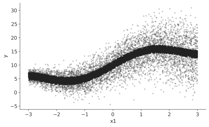
Figure 2.1 shows the simulated population. The mean curve combines a sine wave with a linear trend. The points are tightly clustered when \(x_1\) is near \(-3\) and much more spread out when \(x_1\) is near 3.

Python

import numpy as np
import pandas as pd

sim = pd.read_csv("data/regression_sim.csv")
feature_cols = ["x1", "x2"]
train = sim[sim.split == "train"].reset_index(drop=True)
cal = sim[sim.split == "cal"].reset_index(drop=True)
test = sim[sim.split == "test"].reset_index(drop=True)
print(sim.shape)
print(train.shape, cal.shape, test.shape)

(6000, 6)
(3000, 6) (1500, 6) (1500, 6)

R

sim <- read.csv("data/regression_sim.csv")
feature_cols <- c("x1", "x2")
train <- sim[sim$split == "train", ]
cal   <- sim[sim$split == "cal", ]
test  <- sim[sim$split == "test", ]
cat(dim(sim), "\n")
cat(nrow(train), nrow(cal), nrow(test), "\n")

6000 6
3000 1500 1500

The model uses 3,000 observations for training. Another 1,500 observations set the conformal cutoff, and the final 1,500 evaluate coverage. With 1,500 calibration scores, the rank resolution is \(1/1501\), or about 0.00067. A smaller calibration set gives a coarser and less stable cutoff.

In this simulation, the rows are independent and all three splits come from the same distribution. Calibration and test outcomes were not used for preprocessing or tuning. These design choices make exchangeability plausible. In an observed data set, a split column alone tells us none of this. We need to know how the observations were collected and divided.

2.4 Fitting the base model

Fit an XGBoost regressor with the same settings in both languages.

Python

import xgboost as xgb
from sklearn.metrics import r2_score

reg = xgb.XGBRegressor(n_estimators=300, max_depth=3, learning_rate=0.05, random_state=0)
reg.fit(train[feature_cols], train["y"])
pred_test = reg.predict(test[feature_cols])
print("test R2:", round(r2_score(test["y"], pred_test), 4))

test R2: 0.5903

R

library(xgboost)

dtrain <- xgb.DMatrix(data = as.matrix(train[, feature_cols]), label = train$y)
reg <- xgb.train(
  params = list(max_depth = 3, eta = 0.05, objective = "reg:squarederror"),
  data = dtrain, nrounds = 300
)
pred_test <- predict(reg, as.matrix(test[, feature_cols]))
r2 <- 1 - sum((test$y - pred_test)^2) / sum((test$y - mean(test$y))^2)
cat("test R2:", round(r2, 4), "\n")

test R2: 0.5903

R² is 0.59 in both languages. The true conditional mean obtains about 0.605 on this test set, so the fitted model is close to the best expected squared-error predictor for these data. Much of the remaining variation cannot be predicted from \(x_1\) and \(x_2\). The intervals will reflect that unavoidable noise.

2.5 Split conformal from packages

Both packages predict the calibration outcomes, calculate absolute residuals, select the finite-sample-corrected quantile, and create the test intervals. The intervals have constant width, so \(\hat q\) is half of that width.

Python

SplitConformalRegressor takes the fitted model, conformalizes it on the calibration data, and returns intervals. mapie.metrics.regression supplies the coverage and width numbers as package functions.

from mapie.regression import SplitConformalRegressor
from mapie.metrics.regression import regression_coverage_score, regression_mean_width_score
from scipy.stats import binomtest

alpha = 0.10
scr = SplitConformalRegressor(estimator=reg, confidence_level=1 - alpha,
                               conformity_score="absolute", prefit=True)
scr.conformalize(cal[feature_cols], cal["y"])
pred_test, y_pis = scr.predict_interval(test[feature_cols])
lo, hi = y_pis[:, 0, 0], y_pis[:, 1, 0]

q_hat = (hi[0] - lo[0]) / 2
print("n_cal:", len(cal), "  q_hat:", round(q_hat, 4))

coverage = regression_coverage_score(test["y"].to_numpy(), y_pis)[0]
width = regression_mean_width_score(y_pis)[0]
print("empirical coverage:", round(coverage, 4))
print("mean interval width:", round(width, 4))

covered = (test["y"].to_numpy() >= lo) & (test["y"].to_numpy() <= hi)
ci = binomtest(int(covered.sum()), len(covered)).proportion_ci(method="wilson")
print("covered:", covered.sum(), "of", len(covered))
print("95% Wilson CI:", round(ci.low, 4), "to", round(ci.high, 4))

n_cal: 1500   q_hat: 6.8865
empirical coverage: 0.914
mean interval width: 13.773
covered: 1371 of 1500
95% Wilson CI: 0.8987 to 0.9272

ImportantA common mistake: calling .fit() on a prefit estimator

SplitConformalRegressor(..., prefit=True) expects the model to already be fitted, and calling .fit() on it anyway raises an error rather than silently refitting:

ValueError: The fit method must be skipped when the prefit parameter is set to True.
Use the conformalize method directly after instanciation.

With prefit=True, go directly to .conformalize(). .fit() is only for the case where MAPIE itself should train the base estimator.

R

probably::int_conformal_split() needs a fitted workflow(), not a bare model. The following code puts the XGBoost model in a workflow() and conformalizes it.

library(workflows)
library(parsnip)
library(probably)

xgb_spec <- boost_tree(trees = 300, tree_depth = 3, learn_rate = 0.05) |>
  set_engine("xgboost") |>
  set_mode("regression")
xgb_wflow <- workflow() |> add_model(xgb_spec) |> add_formula(y ~ x1 + x2)
xgb_fit <- fit(xgb_wflow, data = train)

split_conf <- int_conformal_split(xgb_fit, cal)
print(split_conf)

Split Conformal inference
preprocessor: formula
model: boost_tree (engine = xgboost)
calibration set size: 1,500

Use `predict(object, new_data, level)` to compute prediction intervals

alpha <- 0.10
pred_probably <- predict(split_conf, test, level = 1 - alpha)
lo <- pred_probably$.pred_lower
hi <- pred_probably$.pred_upper
q_hat <- (hi[1] - lo[1]) / 2
cat("n_cal:", nrow(cal), "  q_hat:", round(q_hat, 4), "\n")

covered <- (test$y >= lo) & (test$y <= hi)
cat("empirical coverage:", round(mean(covered), 4), "\n")
cat("mean interval width:", round(mean(hi - lo), 4), "\n")

ci <- prop.test(sum(covered), length(covered), correct = FALSE)$conf.int
cat("covered:", sum(covered), "of", length(covered), "\n")
cat("95% score CI:", round(ci[1], 4), "to", round(ci[2], 4), "\n")

n_cal: 1500   q_hat: 6.8865
empirical coverage: 0.914
mean interval width: 13.773
covered: 1371 of 1500
95% score CI: 0.8987 to 0.9272

Both packages give \(\hat q=6.8865\), because they perform the same calculation on the same fitted model and calibration data. The intervals cover 1,371 of the 1,500 test outcomes, or 91.4%, and have mean width 13.77. The 95% Wilson interval for coverage runs from 89.9% to 92.7%. The observed coverage is therefore consistent with a target of 90%.

The uncertainty interval measures how precisely this test set estimates coverage. A different calibration sample could also produce a different cutoff.

NoteHow to interpret coverage

Across comparable future cases, the method is designed to cover at least 90% of outcomes. It does not assign a 90% posterior probability to each interval. It also does not promise 90% coverage in every part of the feature space.

2.6 Diagnose where marginal coverage hides problems

An overall coverage of 90% can hide large differences across the data. We inspect \(x_1\) because the simulation makes the noise increase with \(x_1\). The code divides the test observations into five bins and calculates coverage in each one.

Python

bins = pd.cut(test["x1"], bins=5)
diag = pd.DataFrame({"bin": bins, "covered": covered, "width": hi - lo})
by_bin = diag.groupby("bin", observed=True).agg(
    n=("covered", "size"), coverage=("covered", "mean"), mean_width=("width", "mean"))
print(by_bin.round(4))

                  n  coverage  mean_width
bin
(-3.005, -1.8]  319    1.0000      13.773
(-1.8, -0.6]    311    0.9968      13.773
(-0.6, 0.6]     256    0.9531      13.773
(0.6, 1.799]    318    0.8491      13.773
(1.799, 2.999]  296    0.7703      13.773

R

bins <- cut(test$x1, breaks = 5)
diag_df <- data.frame(bin = bins, covered = covered, width = hi - lo)
by_bin <- diag_df |> dplyr::group_by(bin) |>
  dplyr::summarise(n = dplyr::n(), coverage = mean(covered), mean_width = mean(width))
print(by_bin)

# A tibble: 5 x 4
  bin              n coverage mean_width
  <fct>        <int>    <dbl>      <dbl>
1 (-3.01,-1.8]   319    1           13.8
2 (-1.8,-0.6]    311    0.997       13.8
3 (-0.6,0.6]     256    0.953       13.8
4 (0.6,1.8]      318    0.849       13.8
5 (1.8,3.01]     296    0.770       13.8

Coverage falls from 100% in the lowest bin of \(x_1\) to 77% in the highest. Every interval has width 13.77. The overall value of 91.4% combines strong overcoverage on the left with strong undercoverage on the right.

Subgroup estimates are uncertain, especially when a group is small. Report the number covered, the group size, and an uncertainty interval. Choose important groups in advance when possible. If a low value appears only after trying many different partitions, confirm it with new data.

Figure 2.2: Test observations, their constant-width interval, and which ones are covered.

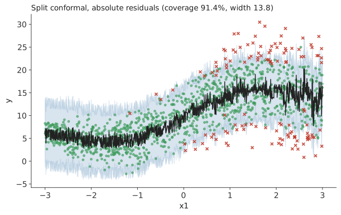
In Figure 2.2, the band is too wide on the left and too narrow on the right. A constant-width interval cannot adapt to the changing noise.

Figure 2.3: Empirical coverage by x1 bin, constant-width split conformal against CQR.

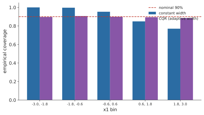
Figure 2.3 also includes the adaptive interval from the next section. Its coverage is closer to 90% in all five bins. This improvement occurs in this example. CQR still does not guarantee conditional coverage.

2.7 Conformalized quantile regression

CQR can help when the outcome spread changes with the features. It estimates lower and upper conditional quantiles, then calibrates those bounds. The coverage guarantee remains marginal. Local coverage depends on how well the quantile models learn the changing spread.

Python

MAPIE’s ConformalizedQuantileRegressor fits lower and upper quantile models from one estimator template. Here the template is a gradient boosting regressor with quantile loss.

from sklearn.ensemble import GradientBoostingRegressor
from mapie.regression import ConformalizedQuantileRegressor

gbr = GradientBoostingRegressor(loss="quantile", alpha=0.5, n_estimators=300,
                                 max_depth=3, learning_rate=0.05, random_state=0)
cqr = ConformalizedQuantileRegressor(estimator=gbr, confidence_level=1 - alpha, prefit=False)
cqr.fit(train[feature_cols], train["y"])
cqr.conformalize(cal[feature_cols], cal["y"])
cqr_pred, cqr_intervals = cqr.predict_interval(test[feature_cols])
cqr_lo, cqr_hi = cqr_intervals[:, 0, 0], cqr_intervals[:, 1, 0]
cqr_covered = (test["y"].to_numpy() >= cqr_lo) & (test["y"].to_numpy() <= cqr_hi)
print("CQR empirical coverage:", round(cqr_covered.mean(), 4))
print("CQR mean interval width:", round((cqr_hi - cqr_lo).mean(), 4))

CQR empirical coverage: 0.896
CQR mean interval width: 11.8859

cqr_diag = pd.DataFrame({"bin": bins, "covered": cqr_covered, "width": cqr_hi - cqr_lo})
print(cqr_diag.groupby("bin", observed=True).agg(
    n=("covered", "size"), coverage=("covered", "mean"), mean_width=("width", "mean")).round(4))

                  n  coverage  mean_width
bin
(-3.005, -1.8]  319    0.8966      5.0642
(-1.8, -0.6]    311    0.9068      8.7304
(-0.6, 0.6]     256    0.8984     11.8725
(0.6, 1.799]    318    0.8931     15.5578
(1.799, 2.999]  296    0.8851     18.6200

Note

MAPIE reports The predictions are ill-sorted. for this fit. For one test observation, the fitted median lies below the fitted lower quantile. The lower and upper quantiles do not cross, and the calibrated interval contains the median. Check this message when it appears. Many ordering problems would indicate that the quantile models need revision.

R

int_conformal_quantile() fits a quantregForest model on train_data to produce the interval bounds. The XGBoost workflow supplies only the point-prediction column. The R and Python examples therefore use different quantile models.

library(dplyr)

set.seed(1)
qc <- int_conformal_quantile(xgb_fit, train_data = train, cal_data = cal, level = 1 - alpha)
print(qc)
pred_qc <- predict(qc, test)
qc_lo <- pred_qc$.pred_lower
qc_hi <- pred_qc$.pred_upper
qc_covered <- (test$y >= qc_lo) & (test$y <= qc_hi)
cat("CQR (probably) empirical coverage:", round(mean(qc_covered), 4), "\n")
cat("CQR (probably) mean interval width:", round(mean(qc_hi - qc_lo), 4), "\n")

Split Conformal inference via Quantile Regression
preprocessor: formula
model: boost_tree (engine = xgboost)
calibration set size: 1,500
confidence level: 0.9

CQR (probably) empirical coverage: 0.9027
CQR (probably) mean interval width: 14.8749

qc_diag <- data.frame(bin = bins, covered = qc_covered, width = qc_hi - qc_lo)
print(qc_diag |> dplyr::group_by(bin) |>
        dplyr::summarise(n = dplyr::n(), coverage = mean(covered), mean_width = mean(width)))

# A tibble: 5 x 4
  bin              n coverage mean_width
  <fct>        <int>    <dbl>      <dbl>
1 (-3.01,-1.8]   319    0.940       12.8
2 (-1.8,-0.6]    311    0.855       13.2
3 (-0.6,0.6]     256    0.957       13.9
4 (0.6,1.8]      318    0.899       16.9
5 (1.8,3.01]     296    0.868       17.5

Overall coverage is 89.6% in Python and 90.3% in R. Both intervals widen as \(x_1\) increases. Python stays near 90% in all five bins. R ranges from 85.5% to 95.7%. Calibration improves marginal coverage, but it does not make the conditional quantiles perfect.

The interval widths differ because the quantile models differ. Python uses gradient boosting. R uses quantregForest. Python’s mean width grows from 5.06 to 18.62 across the bins. R’s grows from 12.8 to 17.5. Compare their coverage and width as two separate fitted methods.

Figure 2.4: Mean interval width by x1 bin, constant-width split conformal against CQR (Python).

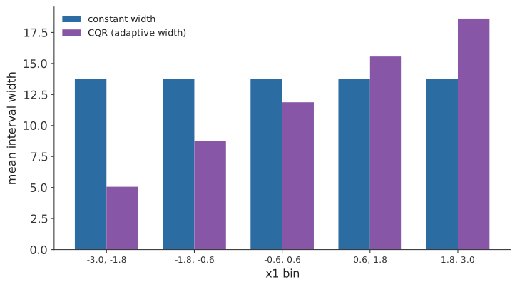
In Figure 2.4, split conformal has the same width in every bin. CQR becomes wider as \(x_1\) increases.

2.8 Inspect the scores and estimate coverage

The calibration scores show the errors used to select the cutoff.

Figure 2.5: Calibration nonconformity scores for the base regression model, with the cutoff used above marked.

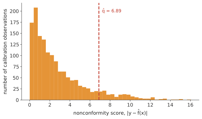
Figure 2.5 uses the calibration residuals from this example. Most are small. The cutoff, \(\hat q=6.8865\), lies in the right tail because the target coverage is 90%.

We can also estimate coverage at several target levels. Large departures from the diagonal would reveal a problem. Points on this curve use the same finite test sample, so they are dependent and uncertain. The curve cannot prove exchangeability.

Python

levels = [0.50, 0.60, 0.70, 0.80, 0.90, 0.95]
scr_multi = SplitConformalRegressor(estimator=reg, confidence_level=levels,
                                     conformity_score="absolute", prefit=True)
scr_multi.conformalize(cal[feature_cols], cal["y"])
_, multi_intervals = scr_multi.predict_interval(test[feature_cols])
for i, lev in enumerate(levels):
    lo_i, hi_i = multi_intervals[:, 0, i], multi_intervals[:, 1, i]
    cov_i = np.mean((test["y"].to_numpy() >= lo_i) & (test["y"].to_numpy() <= hi_i))
    print(f"nominal {lev:.2f}  ->  empirical {cov_i:.4f}")

nominal 0.50  ->  empirical 0.4793
nominal 0.60  ->  empirical 0.5860
nominal 0.70  ->  empirical 0.6947
nominal 0.80  ->  empirical 0.7953
nominal 0.90  ->  empirical 0.9140
nominal 0.95  ->  empirical 0.9613

R

The same check, one confidence level at a time, calling predict() on the already-conformalized split_conf object for each level.

levels <- c(0.50, 0.60, 0.70, 0.80, 0.90, 0.95)
for (lev in levels) {
  pred_lev <- predict(split_conf, test, level = lev)
  cov_lev <- mean(test$y >= pred_lev$.pred_lower & test$y <= pred_lev$.pred_upper)
  cat(sprintf("nominal %.2f  ->  empirical %.4f\n", lev, cov_lev))
}

nominal 0.50  ->  empirical 0.4793
nominal 0.60  ->  empirical 0.5860
nominal 0.70  ->  empirical 0.6947
nominal 0.80  ->  empirical 0.7953
nominal 0.90  ->  empirical 0.9140
nominal 0.95  ->  empirical 0.9613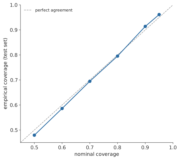

Figure 2.6: Nominal against empirical coverage, six confidence levels, on the test set.

Figure 2.6 compares the target and observed coverage. All six points are close to the diagonal. They will not fall on it perfectly in a finite test sample. Report the number covered, the sample size, and an uncertainty interval for each point. For clustered data, calculate uncertainty at the level of the independent unit.

This is not a probability reliability diagram. It measures how often intervals contain outcomes. It does not test whether events assigned probability 0.70 occur 70% of the time.

TipRepeating the simulation

With simulated data, we can repeat the full train, calibration, and test experiment many times. The resulting distribution of coverage shows the method’s long-run behavior. Repeated splits of one observed data set can test sensitivity to the split, but they do not create new observations.

2.9 The classification simulation

The classification example has four overlapping classes. It was generated with scikit-learn’s make_classification and saved so that R and Python use the same rows.

If your problem is regression, you can skip to the final checklist. Classification uses the same rules for splitting, calibration, and evaluation. Its output is a set of labels, and its main efficiency measure is set size.

Python

simc = pd.read_csv("data/classification_sim.csv")
feat_c = [c for c in simc.columns if c.startswith("x")]
trainc = simc[simc.split == "train"].reset_index(drop=True)
calc = simc[simc.split == "cal"].reset_index(drop=True)
testc = simc[simc.split == "test"].reset_index(drop=True)
print(simc.shape, trainc.shape, calc.shape, testc.shape)

(6000, 8) (3000, 8) (1500, 8) (1500, 8)

R

simc <- read.csv("data/classification_sim.csv")
feat_c <- grep("^x", names(simc), value = TRUE)
trainc <- simc[simc$split == "train", ]
calc_df <- simc[simc$split == "cal", ]
testc <- simc[simc$split == "test", ]
cat(dim(simc), nrow(trainc), nrow(calc_df), nrow(testc), "\n")

6000 8 3000 1500 1500

2.10 Fitting a base classifier

Fit the same XGBoost classifier in both languages. LAC, APS, and RAPS all start from its class probabilities.

Python

clf = xgb.XGBClassifier(n_estimators=300, max_depth=3, learning_rate=0.05,
                         random_state=0, eval_metric="mlogloss")
clf.fit(trainc[feat_c], trainc["y"])
acc = (clf.predict(testc[feat_c]) == testc["y"]).mean()
print("test accuracy:", round(acc, 4))

test accuracy: 0.8907

R

dtrain_c <- xgb.DMatrix(data = as.matrix(trainc[, feat_c]), label = trainc$y)
clf <- xgb.train(
  params = list(max_depth = 3, eta = 0.05, objective = "multi:softprob", num_class = 4,
                eval_metric = "mlogloss"),
  data = dtrain_c, nrounds = 300
)
proba_test_r <- predict(clf, as.matrix(testc[, feat_c]))
pred_label <- max.col(proba_test_r) - 1
cat("test accuracy:", round(mean(pred_label == testc$y), 4), "\n")

test accuracy: 0.8907

Note

Recent versions of R’s xgboost return multiclass probabilities as an n_obs by n_class matrix. Do not reshape this matrix into a vector. Check that rowSums() is close to 1.

2.11 Conformal p-values for one observation

The LAC score for candidate class \(y\) is \(1-\hat\pi_y(x)\). Its conformal p-value compares that score with the calibration scores.

Python

MAPIE returns prediction sets rather than conformal p-values. To locate each p-value, request prediction sets at confidence levels from 1% to 99%. A class enters the set when \(\alpha\) falls below its p-value. Steps of 0.01 locate the p-value within a range of width 0.01.

from mapie.classification import SplitConformalClassifier

row = 0
levels = np.round(np.arange(0.01, 1.00, 0.01), 2).tolist()
scc_sweep = SplitConformalClassifier(estimator=clf, confidence_level=levels,
                                      conformity_score="lac", prefit=True, random_state=0)
scc_sweep.conformalize(calc[feat_c], calc["y"])
_, sets_sweep = scc_sweep.predict_set(testc[feat_c].iloc[[row]])
membership_row = sets_sweep[0]
proba_row = clf.predict_proba(testc[feat_c].iloc[[row]])[0]

for class_idx in range(4):
    included = np.where(membership_row[class_idx] == 1)[0]
    if len(included) == 0:
        bracket = "p-value < 0.01"
    else:
        first = included[0]
        lo_p = round(1 - levels[first], 2)
        hi_p = round(1 - levels[first - 1], 2) if first > 0 else 1.00
        bracket = f"p-value in ({lo_p:.2f}, {hi_p:.2f}]"
    print(f"class {class_idx}: probability={proba_row[class_idx]:.4f}  {bracket}")

class 0: probability=0.0116  p-value < 0.01
class 1: probability=0.0367  p-value in (0.01, 0.02]
class 2: probability=0.9503  p-value in (0.62, 0.63]
class 3: probability=0.0014  p-value < 0.01

R

In R, conformal_pvalue() takes the calibration scores and the four candidate scores. The fitted predictset object contains the scores and the classifier needed for the new probabilities. make_model() connects XGBoost to predictset. The same model wrapper and data split are reused below.

library(predictset)

xgb_clf <- make_model(
  train_fun = function(x, y) {
    d <- xgb.DMatrix(data = as.matrix(x), label = as.integer(y) - 1)
    xgb.train(params = list(max_depth = 3, eta = 0.05, objective = "multi:softprob",
                             num_class = nlevels(y), eval_metric = "mlogloss"),
              data = d, nrounds = 300)
  },
  predict_fun = function(object, x_new) {
    p <- predict(object, as.matrix(x_new))
    colnames(p) <- levels(simc$y)  # predictset matches columns to class labels by name
    p
  },
  type = "classification"
)

simc$y <- factor(simc$y)
trainval <- simc[simc$split %in% c("train", "cal"), ]  # predictset does its own internal cal split
test <- simc[simc$split == "test", ]

row1 <- test[1, feat_c, drop = FALSE]
res <- conformal_lac(trainval[, feat_c], trainval$y, model = xgb_clf, x_new = row1,
                      alpha = 0.10, cal_fraction = 0.33, seed = 1)

proba_row <- res$model$predict_fun(res$fitted_model, row1)[1, ]
p_values <- conformal_pvalue(res$scores, 1 - proba_row)

for (class_idx in 0:3) {
  cat(sprintf("class %d: probability=%.4f  conformal p-value=%.4f\n",
              class_idx, proba_row[class_idx + 1], p_values[class_idx + 1]))
}

class 0: probability=0.0161  conformal p-value=0.0074
class 1: probability=0.0585  conformal p-value=0.0121
class 2: probability=0.9241  conformal p-value=0.5565
class 3: probability=0.0012  conformal p-value=0.0027

For a 90% prediction set, \(\alpha=0.10\). In both languages, class 2 is the only one whose conformal p-value is above 0.10, so the prediction set is \(\{2\}\). Classes 0, 1, and 3 are excluded. A p-value near 0.6 is not a 60% probability that class 2 is correct.

R gives different numbers because predictset fits a new classifier and makes a new calibration split. Compare which classes pass \(\alpha=0.10\), not the exact p-values across languages.

NoteHow to interpret a prediction set

If the set is \(\{1,2\}\), the method is not assigning 90% probability to each class or dividing 90% between them. It returns a set from a method designed to include the true label for 90% of comparable future cases.

2.12 LAC, APS and RAPS in Python

from mapie.classification import SplitConformalClassifier

results = {}
for score in ["lac", "aps", "raps"]:
    scc = SplitConformalClassifier(estimator=clf, confidence_level=0.90,
                                    conformity_score=score, prefit=True, random_state=0)
    scc.conformalize(calc[feat_c], calc["y"])
    labels, sets = scc.predict_set(testc[feat_c])
    membership = sets[:, :, 0]
    sizes = membership.sum(axis=1)
    covered_c = membership[np.arange(len(testc)), testc["y"].to_numpy()]
    results[score] = (membership, sizes, covered_c)
    print(f"{score.upper()}: coverage={covered_c.mean():.4f}  mean size={sizes.mean():.4f}  "
          f"singleton frac={np.mean(sizes==1):.4f}  empty frac={np.mean(sizes==0):.4f}")

LAC: coverage=0.9107  mean size=1.0427  singleton frac=0.9533  empty frac=0.0020
APS: coverage=0.9747  mean size=1.4160  singleton frac=0.6060  empty frac=0.0000
RAPS: coverage=0.9760  mean size=1.4267  singleton frac=0.5967  empty frac=0.0000

TipCompare coverage and set size

LAC covers 91.1% of test labels and returns one class for 95.3% of cases. APS and RAPS cover about 97.5% and return larger sets. On this four-class example, their cumulative-probability scores are conservative. Results can differ with more classes or different RAPS settings. LAC returns an empty set for 0.2% of cases. Report whether the software allows empty sets.

Figure 2.7: Prediction set size distribution for LAC, APS, and RAPS.

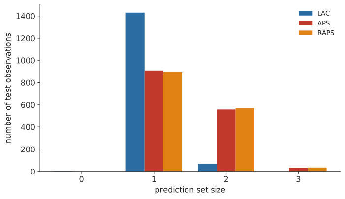
Figure 2.7 shows how often each method returns zero, one, two, or three classes. LAC nearly always returns one class. APS and RAPS often return two and sometimes return three.

Figure 2.8: Coverage by true class and by prediction set size, for APS.

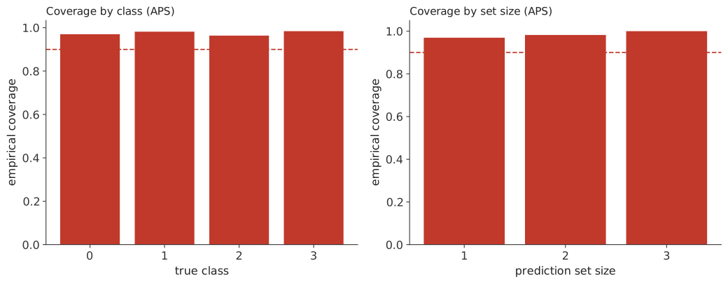
The left panel of Figure 2.8 gives APS coverage for each true class. All four values are at least 90%. The right panel groups observations by prediction-set size. Coverage rises with set size in this test sample and reaches 100% for sets of size 3.

Figure 2.9: APS applied to one test observation: sorted class probabilities and their cumulative sum.

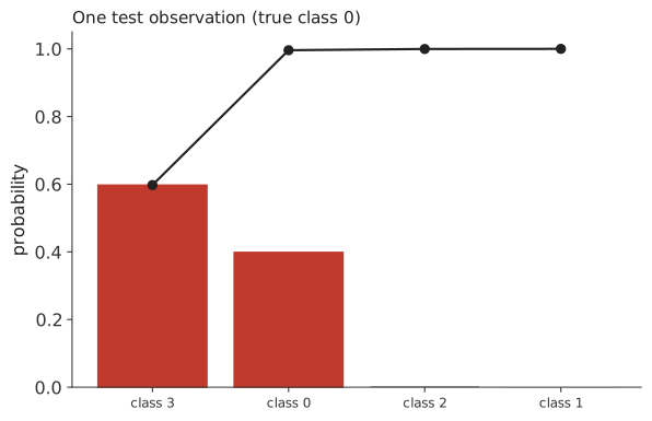
For the observation in Figure 2.9, the two largest probabilities are 0.5975 and 0.3985. The cumulative score does not pass the calibrated cutoff until the second class is added, so APS returns both classes.

2.13 LAC, APS and RAPS in R with predictset

Use the model wrapper and data split created above. predictset handles calibration, calculates the scores, and builds the sets.

for (meth in c("lac", "aps", "raps")) {
  fit_fn <- switch(meth, lac = conformal_lac, aps = conformal_aps, raps = conformal_raps)
  res <- fit_fn(trainval[, feat_c], trainval$y, model = xgb_clf, x_new = test[, feat_c],
                alpha = 0.10, cal_fraction = 0.33, seed = 1)
  cat(sprintf("%s: coverage=%.4f mean size=%.4f singleton frac=%.4f\n",
              toupper(meth), coverage(res, test$y), mean(set_size(res)), mean(set_size(res) == 1)))
}

LAC: coverage=0.9047 mean size=1.0260 singleton frac=0.9740
APS: coverage=0.9447 mean size=1.2247 singleton frac=0.7840
RAPS: coverage=0.9427 mean size=1.2100 singleton frac=0.7947

These R values cannot be compared line by line with the Python values. predictset fits a new XGBoost model and makes a new calibration split from the combined training and calibration rows. MAPIE uses the earlier fitted model and the fixed calibration rows. Both the model and the split have changed.

For a fair method comparison, keep the fitted model, data split, target coverage, and test cases fixed.

2.14 What the diagnostics can tell you

The diagnostics used throughout this chapter answer different questions:

For regression:

Diagnostic	Question it answers
Empirical coverage, count, and uncertainty interval	How precisely does this evaluation sample estimate marginal coverage?
Mean, median, and distribution of interval width	How informative are the intervals, and do a few very wide intervals dominate the mean?
Coverage by a pre-specified feature or group	Is there evidence of practically important heterogeneity hidden by the marginal average?
Calibration score histogram	What do held-out prediction errors look like, and where does the selected cutoff fall?
Nominal vs. empirical coverage curve	Is there a broad discrepancy across several target levels on this evaluation sample?

For classification:

Diagnostic	Question it answers
Prediction-set coverage, count, and uncertainty interval	How precisely does this sample estimate marginal label coverage?
Set-size distribution, empty and singleton fractions	How informative or indecisive are the sets?
Coverage by a pre-specified class or group	Is there evidence that important classes or populations are undercovered?
Coverage by set size	How does observed coverage vary with the method’s degree of caution?
Per-class conformal p-values for an example	Which candidate labels does the calibrated rule reject at the selected \(\alpha\)?
APS cumulative probability display	How does a ranked probability vector become a prediction set?

Ordinary conformal prediction controls overall coverage. The subgroup, width, set-size, and shift checks help find problems, but they do not come with the same guarantee.

2.15 What to report

Before reporting a conformal result, record:

1. Prediction problem: observational unit, outcome or label, target population, and information available at prediction time.
2. Data design: training, validation, calibration, and test sizes. Include the random seed and whether splitting was by row, person, cluster, site, or time.
3. Final method: base model and preprocessing, conformity score, target coverage, software version, treatment of ties and randomization, and whether empty classification sets are allowed.
4. Why the split is suitable: why calibration cases are comparable to future cases, plus known dependence or shift concerns.
5. Coverage: number covered, denominator, empirical coverage, and an uncertainty interval on untouched evaluation data.
6. Efficiency: interval-width distribution or prediction-set-size distribution, not only its mean.
7. Planned subgroup checks: coverage and efficiency in groups that matter for the research question, with group sizes and uncertainty.
8. Deployment plan: how covariate and conformity-score drift will be monitored and when calibration will be refreshed.

2.16 Common mistakes

Mistake	Better practice
Calibrating on training residuals, or tuning on calibration data	Learn every model and design choice first. Use an untouched calibration sample
Choosing the winning method after inspecting final test results	Select on training and validation data, freeze the method, and evaluate once
Randomly splitting repeated, clustered, or time-ordered rows	Split at the independent unit and in the direction predictions will be made
Treating a non-significant shift check as proof of exchangeability	Combine design knowledge with covariate checks and later score monitoring. Failure to detect shift is not proof that no shift exists
Reading 90% marginal coverage as a 90% probability for each interval or as 90% coverage in every subgroup	Describe 90% as the long-run overall rate and report subgroup coverage separately
Confusing class probabilities, conformal p-values, and probability calibration	Interpret each quantity separately. Conformal label coverage does not calibrate class probabilities
Reporting coverage without uncertainty or efficiency	Give the count, denominator, uncertainty interval, and width or set-size distribution
Assuming CQR or finer Mondrian groups automatically solve conditional coverage	Check coverage with adequate group sizes. Neither method guarantees coverage at every feature value

Calibration size also deserves an explicit calculation. The attainable tail resolution is \(1/(n_{cal}+1)\). A finite split-conformal cutoff for miscoverage \(\alpha\) requires roughly \(n_{cal} \ge 1/\alpha-1\), but this mathematical minimum may give a highly variable cutoff. Choose the sample size using the target level, required precision, subgroup needs, and score variability.