3 The mathematics of conformal prediction
3.1 One fitted model and nine calibration errors
Let \(\hat f\) denote a fitted regression model. For features \(x\), it produces the point prediction \(\hat f(x)\). The hat is a reminder that the function was estimated from training data.
The model has already been trained. We now give it nine observations that were not used during fitting. These form the calibration set:
\[ (X_1,Y_1),\ldots,(X_9,Y_9). \]
\(X_i\) contains the features for row \(i\), and \(Y_i\) is its observed outcome. For each row, calculate the absolute prediction error
\[ S_i=\left|Y_i-\hat f(X_i)\right|. \]
The letter \(S\) stands for score. A small score means the prediction was close; a large score means it was far away.
| \(i\) | prediction \(\hat f(X_i)\) | outcome \(Y_i\) | residual \(Y_i-\hat f(X_i)\) | score \(S_i\) |
|---|---|---|---|---|
| 1 | 98 | 99 | 1 | 1 |
| 2 | 102 | 104 | 2 | 2 |
| 3 | 95 | 92 | \(-3\) | 3 |
| 4 | 107 | 111 | 4 | 4 |
| 5 | 90 | 85 | \(-5\) | 5 |
| 6 | 100 | 106 | 6 | 6 |
| 7 | 93 | 100 | 7 | 7 |
| 8 | 110 | 102 | \(-8\) | 8 |
| 9 | 96 | 108 | 12 | 12 |
The scores are already sorted here:
\[ 1,2,3,4,5,6,7,8,12. \]
Nothing conformal has happened yet. We have only measured how the fitted model behaved on data it did not train on.
The model and every preprocessing step must be fixed before these scores are calculated. If calibration outcomes are used to tune the model, choose features, or select a score, the simple split-conformal guarantee below no longer applies directly.
3.2 Try a possible value for a new outcome
A new observation arrives with features \(x_*\). The star marks the new case. Suppose the model predicts
\[ \hat f(x_*)=100. \]
Its true outcome, \(Y_*\), has not been observed. Start by trying \(y=104\) as a possible outcome. If 104 were correct, its score would be
\[ S(x_*,104)=|104-100|=4. \]
Six calibration scores are at least this large: \(4,5,6,7,8,12\). An error of 4 is therefore ordinary for this model.
Now try two values farther from the prediction:
\[ S(x_*,108)=|108-100|=8, \]
which only two calibration scores match or exceed, and
\[ S(x_*,150)=|150-100|=50, \]
which is larger than every calibration score. The farther a candidate moves from 100, the less it resembles the errors seen during calibration.
3.3 Turn that comparison into a conformal p-value
For any candidate outcome \(y\), count the calibration scores that are at least as large as the candidate’s score. Then add the candidate itself to both the count and the sample size:
\[ p(y)=\frac{1+\sum_{i=1}^{n}\mathbf 1\{S_i\geq S(x_*,y)\}}{n+1}. \]
The indicator \(\mathbf 1\{\cdot\}\) equals 1 when the condition inside the braces is true and 0 otherwise. The sum is therefore just a count.
For the three candidates above, with \(n=9\),
\[ p(104)=\frac{1+6}{10}=0.7, \qquad p(108)=\frac{1+2}{10}=0.3, \qquad p(150)=\frac{1+0}{10}=0.1. \]
Read a conformal p-value as a rank comparison:
- A large value means the candidate’s error would not look unusual beside the calibration errors.
- A small value means the candidate would require an unusually large error.
It is not the probability that \(Y_*=y\). For example, \(p(104)=0.7\) does not mean there is a 70% chance that the outcome equals 104.
Why add 1? The candidate is being ranked together with the \(n\) calibration scores. There are \(n+1\) scores in that comparison, so the smallest possible p-value is \(1/(n+1)\) rather than zero.
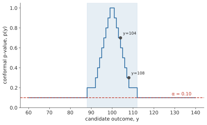
The curve in Figure 3.1 changes in steps because the count changes only when the candidate score passes one of the nine calibration scores. It is symmetric around 100 because absolute error treats values equally far above and below the prediction in the same way.
3.4 Keep the candidates that are not too unusual
Let \(\alpha\) be the allowed error rate. For 90% target coverage, \(\alpha=0.10\). Keep every candidate with a conformal p-value greater than \(\alpha\):
\[ C_\alpha(x_*)=\{y:p(y)>\alpha\}. \]
For the running example, candidates from 88 through 112 survive. At either endpoint the score is 12 and the p-value is 0.2. Moving even slightly farther away produces a score above 12 and a p-value of 0.1, which is not greater than \(\alpha\). Thus
\[ C_{0.10}(x_*)=[88,112]. \]
This candidate-by-candidate view explains the logic, but regression intervals can be computed more directly.
3.5 Compute the same interval with one quantile
Write the sorted scores as
\[ S_{(1)}\leq S_{(2)}\leq\cdots\leq S_{(n)}. \]
Choose the rank
\[ k=\left\lceil(n+1)(1-\alpha)\right\rceil, \]
where \(\lceil z\rceil\) means round \(z\) up to the next integer. Then take
\[ \hat q=S_{(k)}. \]
For \(n=9\) and \(\alpha=0.10\),
\[ k=\lceil 10\times0.90\rceil=9, \qquad \hat q=S_{(9)}=12. \]
Keep any candidate whose error is no larger than \(\hat q\):
\[ |y-\hat f(x_*)|\leq\hat q. \]
Removing the absolute value gives
\[ \hat f(x_*)-\hat q\leq y\leq\hat f(x_*)+\hat q. \]
Therefore
\[ C_\alpha(x_*)= \left[\hat f(x_*)-\hat q,\ \hat f(x_*)+\hat q\right] =[100-12,100+12]=[88,112]. \]
The p-value route and the quantile route produce the same interval. Software uses the quantile route because it avoids checking every possible value of \(y\).
3.6 Why the interval covers often enough
The proof uses one idea: if the calibration cases and the new case are interchangeable, the new score has no preferred position in their combined ranking.
3.6.1 The assumption: exchangeability
After conditioning on the training data, the fitted model \(\hat f\) is fixed. We require the \(n\) calibration observations and the new observation to be exchangeable. Roughly, their order should carry no information about which one becomes the new case.
Independent observations drawn from the same population are exchangeable. Repeated measurements from one patient, a chronological series, or observations collected from different populations may not be.
Random variables \(Z_1,\ldots,Z_m\) are exchangeable when reordering them does not change their joint distribution. For every permutation \(\pi\),
\[ (Z_1,\ldots,Z_m)\stackrel d= (Z_{\pi(1)},\ldots,Z_{\pi(m)}). \]
The symbol \(\stackrel d=\) means “has the same probability distribution as.” Independent and identically distributed observations satisfy this condition, although exchangeability is slightly more general than independence.
3.6.2 Rank the new score with the calibration scores
Imagine that the new outcome has now been observed. Calculate its score in exactly the same way:
\[ S_{n+1}=|Y_{n+1}-\hat f(X_{n+1})|. \]
Place it beside the calibration scores:
\[ S_1,\ldots,S_n,S_{n+1}. \]
Because the same fixed scoring rule is used for every exchangeable observation, the scores are also exchangeable. If there are no ties, the new score is equally likely to occupy any of the \(n+1\) ranks.
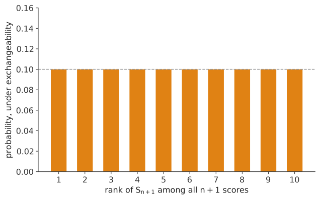
For the nine-row example, Figure 3.2 shows ten possible ranks, each with probability \(1/10\).
The interval misses when the new score is larger than the calibration cutoff \(S_{(k)}\). Without ties, that happens when the new score’s rank among all \(n+1\) scores exceeds \(k\). Hence
\[ P(\text{miss})=\frac{n+1-k}{n+1}. \]
Since
\[ k=\left\lceil(n+1)(1-\alpha)\right\rceil \geq(n+1)(1-\alpha), \]
we obtain
\[ P(\text{miss}) =\frac{n+1-k}{n+1} \leq\alpha. \]
Equivalently,
\[ P\{Y_{n+1}\in C_\alpha(X_{n+1})\}\geq1-\alpha. \]
That is the split-conformal coverage result.
With ties, an ordinary rank is not exactly uniform. Counting scores with \(S_i\geq S_{n+1}\) and using the strict rule \(p(y)>\alpha\) makes the procedure conservative: coverage does not fall below the bound. Random tie-breaking can recover exact rank uniformity when exactness is needed.
The predictive model does not need to be correct for this proof. A poor model produces larger scores and therefore wider intervals, but the rank calculation is unchanged. What must remain credible is the exchangeability of calibration and future scores, with the fitted model and score fixed before calibration.
3.7 How to read the guarantee
The probability above averages over a fresh calibration sample and a fresh future observation from the population. It is marginal coverage:
\[ P\{Y\in C_\alpha(X)\}\geq1-\alpha. \]
It does not generally give 90% coverage at every feature value:
\[ P\{Y\in C_\alpha(X)\mid X=x\}\geq1-\alpha \quad\text{for every }x. \]
The second display is a much stronger requirement and ordinary split conformal does not provide it.
For example, suppose one group contains 600 observations with 96.2% coverage and another contains 200 observations with 68.5% coverage. The pooled coverage is
\[ \frac{600(0.962)+200(0.685)}{800}=0.8928. \]
The overall number is close to 90%, even though the smaller group is poorly covered. This is why coverage should also be inspected in scientifically important groups. Such diagnostics reveal problems; they do not turn the marginal guarantee into pointwise conditional coverage.
A 90% interval should also not be read as “this particular realized interval has a 90% probability of containing its already-fixed outcome.” The 90% describes the repeated performance of the procedure.
3.8 Small calibration samples limit what is possible
With \(n\) calibration observations, conformal p-values lie on the grid
\[ \frac1{n+1},\frac2{n+1},\ldots,1. \]
For \(n=9\), the spacing is 0.1. That is why the 90% interval had to use the largest calibration score.
For a 95% target with the same nine observations,
\[ k=\lceil10(0.95)\rceil=10. \]
There is no tenth calibration score. The finite-sample convention is \(\hat q=\infty\), which returns the whole real line. Nine observations cannot support a finite distribution-free 95% interval.
More generally, a finite cutoff requires approximately
\[ n\geq\frac1\alpha-1. \]
| target coverage | \(\alpha\) | smallest possible \(n\) for a finite cutoff |
|---|---|---|
| 90% | 0.10 | 9 |
| 95% | 0.05 | 19 |
| 99% | 0.01 | 99 |
These are mathematical minima, not recommended sample sizes. At the minimum, the cutoff is the single largest score and can vary greatly from one calibration sample to another. Larger samples give a finer rank grid and a more stable tail estimate. If scores are calibrated separately within groups, the relevant \(n\) is the calibration count inside each group.
3.9 Change the score to change the interval
The proof only needs the same pre-specified score for calibration and future observations. It does not require absolute error. Different scores produce intervals with different shapes and efficiency.
3.9.1 Asymmetric errors
Absolute error gives the same allowance above and below the prediction. If underprediction and overprediction behave differently, use two one-sided scores:
\[ S_i^{\mathrm{lo}}=\hat f(X_i)-Y_i, \qquad S_i^{\mathrm{hi}}=Y_i-\hat f(X_i). \]
Calibrate each tail at level \(\alpha/2\), obtaining \(\hat q_{\mathrm{lo}}\) and \(\hat q_{\mathrm{hi}}\). The interval becomes
\[ \left[ \hat f(x_*)-\hat q_{\mathrm{lo}}, \ \hat f(x_*)+\hat q_{\mathrm{hi}} \right]. \]
The two widths can differ. Splitting the error budget across the tails ensures total miscoverage of at most \(\alpha\) by the union bound.
3.9.2 Normalized scores
A single absolute-error cutoff gives every observation the same width. That is inefficient when the outcome is much noisier in some regions than others.
Let \(\hat\sigma(x)>0\) estimate the local size of a typical error. It must be fitted without using calibration outcomes. Define
\[ S_i=\frac{|Y_i-\hat f(X_i)|}{\hat\sigma(X_i)}. \]
Calibrate these normalized scores exactly as before. For a new observation,
\[ \frac{|y-\hat f(x_*)|}{\hat\sigma(x_*)}\leq\hat q \]
gives
\[ C_\alpha(x_*)= \left[ \hat f(x_*)-\hat q\hat\sigma(x_*), \ \hat f(x_*)+\hat q\hat\sigma(x_*) \right]. \]
The interval is wider where \(\hat\sigma(x_*)\) is large. Marginal validity still follows from the rank proof. A poor scale model does not invalidate that proof, but it allocates width poorly and can leave large subgroup differences.
3.9.3 Conformalized quantile regression
Conformalized quantile regression (CQR) starts with two conditional quantile estimates rather than a point prediction and a scale model. For target coverage \(1-\alpha\), fit
\[ \hat Q_{\alpha/2}(x) \quad\text{and}\quad \hat Q_{1-\alpha/2}(x) \]
on training data. These estimate a lower and upper boundary for the outcome distribution.
For calibration row \(i\), use
\[ S_i=\max\left\{ \hat Q_{\alpha/2}(X_i)-Y_i, \ Y_i-\hat Q_{1-\alpha/2}(X_i) \right\}. \]
The score is positive when the outcome falls outside the initial interval. It can be negative when the outcome lies inside it.
Suppose every calibration row has initial bounds \([90,110]\). This is deliberately simplified; normally the bounds vary with \(X_i\).
| \(i\) | lower | upper | \(Y_i\) | CQR score |
|---|---|---|---|---|
| 1 | 90 | 110 | 100 | \(-10\) |
| 2 | 90 | 110 | 92 | \(-2\) |
| 3 | 90 | 110 | 108 | \(-2\) |
| 4 | 90 | 110 | 85 | 5 |
| 5 | 90 | 110 | 115 | 5 |
| 6 | 90 | 110 | 80 | 10 |
| 7 | 90 | 110 | 120 | 10 |
| 8 | 90 | 110 | 75 | 15 |
| 9 | 90 | 110 | 99 | \(-9\) |
The sorted scores are
\[ -10,-9,-2,-2,5,5,10,10,15. \]
At 90% coverage with \(n=9\), \(\hat q=15\). If the new row has initial quantile bounds \([92,118]\), conformalization gives
\[ \left[ \hat Q_{\alpha/2}(x_*)-\hat q, \ \hat Q_{1-\alpha/2}(x_*)+\hat q \right] =[77,133]. \]
If \(\hat q\) is negative, the calibrated interval becomes narrower. If it is positive, the interval becomes wider. CQR retains marginal coverage under exchangeability, but it does not guarantee conditional coverage or narrower intervals. Its benefit comes when the fitted quantiles successfully learn how the outcome spread changes with \(x\).
3.10 Classification: from one label to a set
A classifier gives a probability for each class:
\[ \hat\pi_y(x)=P_{\mathrm{model}}(Y=y\mid X=x). \]
These model probabilities are ingredients for a conformity score. They are not conformal p-values.
3.10.1 LAC: score each class by its own probability
Least Ambiguous Classifier (LAC) uses
\[ S(x,y)=1-\hat\pi_y(x). \]
A class with high model probability receives a small score. On calibration row \(i\), score only the true class:
\[ S_i=1-\hat\pi_{Y_i}(X_i). \]
| \(i\) | probability assigned to the true class | LAC score |
|---|---|---|
| 1 | 0.92 | 0.08 |
| 2 | 0.55 | 0.45 |
| 3 | 0.81 | 0.19 |
| 4 | 0.40 | 0.60 |
| 5 | 0.67 | 0.33 |
| 6 | 0.73 | 0.27 |
| 7 | 0.29 | 0.71 |
| 8 | 0.88 | 0.12 |
| 9 | 0.61 | 0.39 |
The sorted scores are \(0.08,0.12,0.19,0.27,0.33,0.39,0.45,0.60,0.71\). Use an 80% target here so the small example does not again select the largest score:
\[ k=\lceil10(0.80)\rceil=8, \qquad \hat q=0.60. \]
For a new case, retain class \(y\) when
\[ 1-\hat\pi_y(x_*)\leq0.60, \]
or equivalently when \(\hat\pi_y(x_*)\geq0.40\). The prediction set contains every class that passes this threshold.
LAC can produce an empty set when no class passes. Some software can force a nonempty set, but that changes the procedure. Report which option was used.
3.10.2 APS: use the whole ranked probability vector
Adaptive Prediction Sets (APS) first sort the probabilities:
\[ \hat\pi_{(1)}(x)\geq\hat\pi_{(2)}(x)\geq\cdots. \]
Suppose four sorted probabilities are
\[ 0.45,\quad0.30,\quad0.20,\quad0.05, \]
with cumulative sums
\[ 0.45,\quad0.75,\quad0.95,\quad1.00. \]
If candidate class \(y\) has rank \(r\), a simple deterministic APS score is
\[ S_{\mathrm{APS}}(x,y)=\sum_{j=1}^{r}\hat\pi_{(j)}(x). \]
The four candidate scores in this example are therefore \(0.45,0.75,0.95,1.00\). Calibration uses the score belonging to each row’s true class. After obtaining \(\hat q\), a new class is included when its candidate score is no larger than \(\hat q\).
A common randomized version replaces the full probability of the candidate class by a random fraction:
\[ S_{\mathrm{APS}}^{\mathrm{rand}}(x,y) =\sum_{j<r}\hat\pi_{(j)}(x)+U\hat\pi_{(r)}(x), \qquad U\sim\operatorname{Uniform}(0,1). \]
This smooths the discrete boundary and can reduce conservative overcoverage. Software differs in whether it randomizes the boundary or always includes the first class that crosses the cumulative cutoff. Those options can change set sizes, so they belong in the method description.
Unlike LAC, APS responds to the entire probability vector. It can return one class when probability is concentrated at the top and several classes when probability is spread across plausible alternatives.
3.10.3 RAPS: discourage very deep sets
Regularized Adaptive Prediction Sets (RAPS) add a penalty for classes far down the ranking:
\[ S_{\mathrm{RAPS}}(x,y) =S_{\mathrm{APS}}(x,y) +\lambda(r-k_{\mathrm{reg}})^+, \]
where \((z)^+=\max(z,0)\). The first \(k_{\mathrm{reg}}\) ranks receive no penalty; later ranks receive an additional \(\lambda\) per position.
For probabilities \(0.35,0.25,0.15,0.10,0.08,0.07\), with \(k_{\mathrm{reg}}=2\) and \(\lambda=0.15\):
| rank | probability | APS cumulative score | penalty | RAPS score |
|---|---|---|---|---|
| 1 | 0.35 | 0.35 | 0.00 | 0.35 |
| 2 | 0.25 | 0.60 | 0.00 | 0.60 |
| 3 | 0.15 | 0.75 | 0.15 | 0.90 |
| 4 | 0.10 | 0.85 | 0.30 | 1.15 |
| 5 | 0.08 | 0.93 | 0.45 | 1.38 |
| 6 | 0.07 | 1.00 | 0.60 | 1.60 |
At the same illustrative cutoff of 0.85, deterministic APS would retain ranks 1 through 4, while these RAPS scores retain only ranks 1 and 2. In a real comparison, however, APS and RAPS must each be calibrated separately. Their cutoffs will generally differ, so RAPS is not guaranteed to produce smaller sets on every problem. Its regularization is most useful with many classes and long probability tails.
3.10.4 Conformal coverage is not probability calibration
For a binary classifier, probability calibration asks whether
\[ P\{Y=1\mid\hat p(X)=p\}\approx p. \]
Among cases assigned probability 0.7, roughly 70% should belong to class 1.
Conformal calibration does something else. It chooses a score cutoff so that the resulting set contains the true label often enough. The rank proof never requires \(\hat\pi_y(x)\) to be a calibrated probability. Better probabilities can still improve efficiency by producing smaller, more informative sets.
3.11 Coverage within pre-defined groups
Suppose every observation belongs to a known group \(G_1,\ldots,G_m\), such as a hospital. Mondrian or group-conditional conformal prediction calculates a separate cutoff inside each group:
\[ \hat q_1,\ldots,\hat q_m. \]
A new observation in group \(g\) uses \(\hat q_g\). If calibration and future scores are exchangeable within that group, the same rank proof gives
\[ P\{Y\in C_\alpha(X)\mid X\in G_g\}\geq1-\alpha. \]
This protects the chosen groups, not every possible value of \(x\). Groups should be defined before calibration. Each group also needs enough calibration data; dividing data into many small cells makes cutoffs unstable or infinite.
3.12 Other ways to reuse limited data
Split conformal is easy to understand and cheap to compute, but it holds data aside for calibration. Other methods trade computation for greater data reuse.
3.12.1 Full conformal prediction
For each candidate outcome \(y\) at \(x_*\):
- append \((x_*,y)\) to the training data;
- refit the model on the augmented data;
- score every training observation and the candidate symmetrically;
- calculate the candidate’s conformal p-value; and
- retain \(y\) when its p-value exceeds \(\alpha\).
Full conformal uses all observations for fitting and comparison, but it may require a new model fit for every candidate value and every new case. That is often impractical for continuous outcomes or expensive models.
3.12.2 The jackknife and Jackknife+
For each observation \(i\), fit a model without that observation, denoted \(\hat f_{-i}\). Its leave-one-out residual is
\[ R_i=|Y_i-\hat f_{-i}(X_i)|. \]
An ordinary jackknife interval combines these residuals with a common full-data prediction. Jackknife+ instead lets every leave-one-out model predict the new case too. Model \(i\) contributes
\[ \hat f_{-i}(x_*)-R_i \quad\text{and}\quad \hat f_{-i}(x_*)+R_i. \]
Finite-sample-adjusted lower and upper quantiles of these \(n\) values form the Jackknife+ interval. Under exchangeability, the basic finite-sample result guarantees coverage of at least \(1-2\alpha\) in general; under additional stability conditions it is typically much closer to the nominal \(1-\alpha\). The price is \(n\) model fits.
3.12.3 CV+
CV+ replaces leave-one-out fits with \(K\) folds. Each model is trained on \(K-1\) folds, scores its held-out fold, and predicts \(x_*\). The resulting lower and upper candidates are combined as in Jackknife+.
CV+ needs \(K\) fits instead of \(n\). When \(K=n\), with one observation per fold, it becomes Jackknife+. Its coverage theory is related to Jackknife+ and should not be described as the exact split-conformal \(1-\alpha\) theorem proved earlier.
| method | model fits | separate calibration set? | main trade-off |
|---|---|---|---|
| Split conformal | 1 | yes | simplest and cheapest, but holds data out |
| Full conformal | many per prediction | no | strong symmetry, usually very expensive |
| Jackknife+ | \(n\) | no fixed split | extensive data reuse, many fits |
| CV+ | \(K\) | no fixed split | compromise between computation and reuse |
3.13 When the ordinary proof no longer applies
3.13.1 Model selection after calibration
The proof treated the fitted model and score as fixed before calibration. Repeatedly checking calibration performance and changing the model, features, score, or target groups makes the calibration scores part of the selection process.
Use training and validation data for those choices. After the full procedure is locked, calculate the calibration scores once. Use a separate test set only for final evaluation.
3.13.2 Distribution shift
If deployment differs from calibration, the new score may no longer have the same rank behavior as the calibration scores.
Under pure covariate shift, the distribution of \(X\) changes while \(Y\mid X\) remains the same. Weighted conformal methods use the density ratio
\[ w(x)=\frac{p_{\mathrm{deploy}}(x)}{p_{\mathrm{cal}}(x)} \]
to give more influence to calibration cases that resemble deployment cases. Exact weighted-conformal results require the shift model and weights to be correct, along with adequate overlap between the two populations. Estimated weights add another source of error. Changes in \(Y\mid X\) cannot be repaired by this covariate-shift weighting alone.
3.13.3 Time series
Time order usually destroys exchangeability: yesterday and tomorrow cannot simply be swapped without changing the data-generating process. Randomly mixing past and future rows can also leak future information into calibration.
Methods such as EnbPI use out-of-block residuals and update them over time. Adaptive Conformal Inference adjusts the working error level after recent misses and coverage successes. These methods have guarantees tailored to sequential data; they do not inherit the ordinary split-conformal proof merely by using a conformal cutoff.