1  Understanding conformal prediction

1.1 Why uncertainty matters

A model is trained to predict how long a patient will need to recover after a procedure. For one patient, it returns 18 days.

The prediction does not show how much recovery times vary among similar patients. A prediction of 18 days could come with a narrow range of plausible outcomes or a range from 5 to 40 days. Those situations require different decisions even though the point prediction is the same.

Figure 1.1: Three patients with the same predicted recovery time, but very different plausible spreads around it.

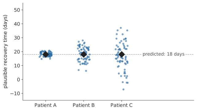
In Figure 1.1, all three patients have a prediction of 18 days, but the plausible spread differs. A point prediction does not show this difference.

The same problem occurs in classification. Consider three class probabilities:

Figure 1.2: A classifier’s probabilities for three classes. A and B are close together, and C is very unlikely.

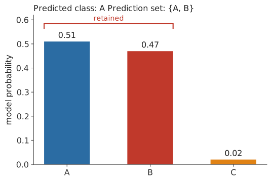
A classifier that returns only the most likely class reports A. In Figure 1.2, A has probability 0.51 and B has probability 0.47. A prediction of 0.51 is much less decisive than a prediction of 0.98, but both cases receive the same label.

Conformal prediction adds a prediction interval in regression or a prediction set in classification. Under the assumptions described below, the interval or set contains the outcome at a chosen long-run rate. The classifier above might return \(\{A, B\}\) rather than only A.

1.2 Intervals, probabilities, and prediction sets

Several forms of uncertainty have different meanings.

A confidence interval describes uncertainty about a fixed but unknown quantity, such as a regression coefficient or population mean.

A prediction interval gives a range for a future or held-out outcome. It concerns an observation of \(Y\), not a model parameter.

A class probability is the probability that a classifier assigns to one class.

A prediction set contains the classes retained by a conformal classifier. Depending on the method and observation, it may contain one class, several classes, no classes, or every class.

Figure 1.3: Point predictions next to their interval or set counterparts, for both regression and classification.

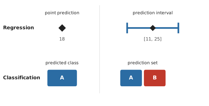
This chapter concerns prediction intervals and prediction sets, not confidence intervals for model parameters.

1.3 Models without prediction intervals

Some models provide prediction intervals under specific assumptions. Classical linear regression is one example. Many predictive models return only a point or class probabilities by default. Variation among random-forest trees is not itself a calibrated prediction interval, and standard gradient-boosting models do not attach an interval to each prediction.

Conformal prediction can be applied to many fitted models, including linear models, random forests, gradient boosting, and neural networks. It uses held-out data to turn their predictions into intervals or sets. The model does not need to provide its own uncertainty estimate.

1.4 Training, calibration and test data

Split conformal prediction assigns separate roles to training, calibration, and test data.

Figure 1.4: Three separate data sets, each doing a different job.

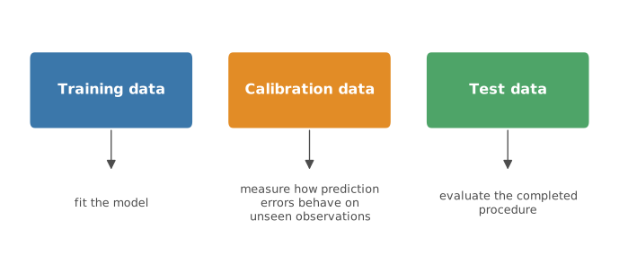
The training data fit the predictive model. The calibration data measure its errors on observations not used for fitting. The test data evaluate the completed model and conformal procedure. Figure 1.4 shows these roles.

Training errors cannot replace calibration errors because the model has already used those observations.

Figure 1.5: Errors on the data a model was trained on are systematically smaller than its errors on genuinely new data.

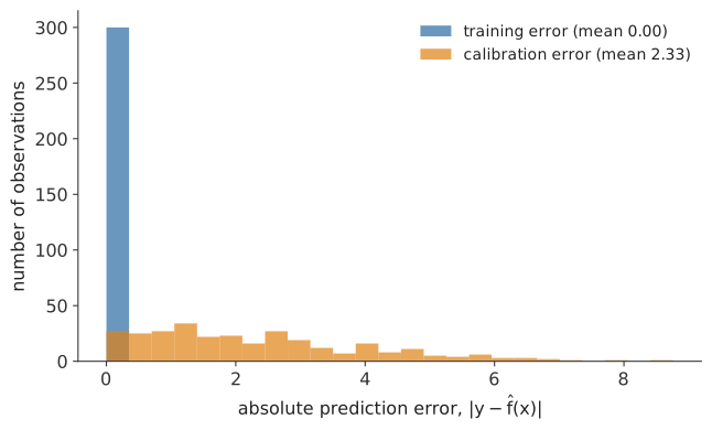
In Figure 1.5, a flexible model nearly memorizes its training data. Its training errors are close to zero, while its errors on unseen calibration observations are much larger. Training residuals are therefore too optimistic for split conformal calibration.

1.5 Probability calibration and conformal calibration

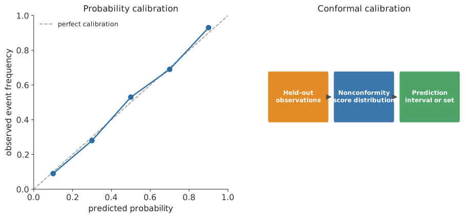
Probability calibration and conformal calibration are different procedures.

Probability calibration compares predicted probabilities with observed frequencies. Among cases assigned probability 0.70, the event should occur about 70% of the time.

Conformal calibration uses scores from held-out observations to determine the size of a prediction interval or set. It does not make class probabilities calibrated and usually does not change the fitted model.

Figure 1.6: Probability calibration and conformal calibration ask different questions.

1.6 Nonconformity scores

A nonconformity score measures disagreement between a prediction and an observed outcome. Small scores indicate better agreement and large scores indicate worse agreement.

The simplest regression score is the absolute residual, the absolute difference between the outcome and its prediction. Quantile regression and classification use other scores, but retain the same direction: smaller means more agreement.

Figure 1.7: The distribution of nonconformity scores across the calibration set, with three example observations placed on it.

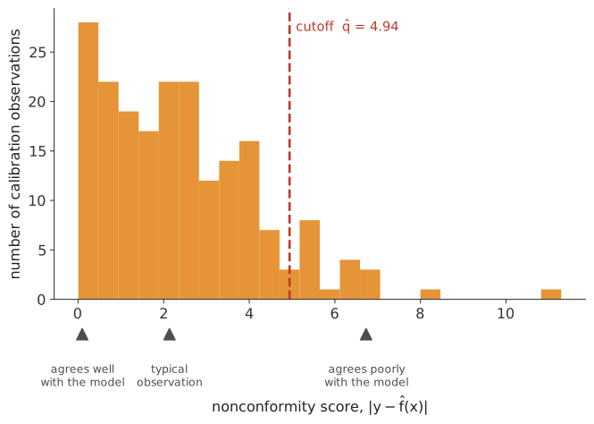
Figure 1.7 shows absolute residuals for 200 calibration observations. The dashed line marks a cutoff, \(\hat q\), selected from these scores.

1.7 Conformal p-values

For a new patient, suppose \(\hat f(x_*)=20\) days. A candidate outcome of 22 has score \(|22-20|=2\).

Compare this score with the calibration scores in Figure 1.7. A candidate far from 20 has a large score. If few calibration scores are at least that large, the candidate is unusual relative to the calibration data.

A conformal p-value is based on the fraction of calibration scores at least as large as the candidate score, with the finite-sample adjustment given in the mathematics chapter. Large values indicate that the candidate is compatible with the calibration scores. Small values indicate that it is unusual.

Figure 1.8: The conformal p-value for candidate outcomes near and far from a new prediction of 20 days.

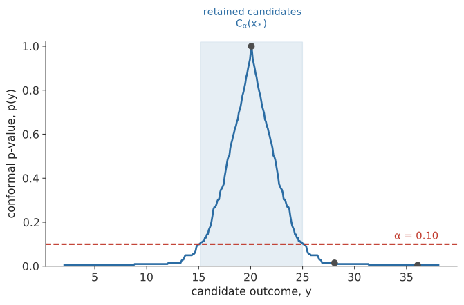
In Figure 1.8, candidates close to 20 have large p-values. The p-value falls as the candidate moves away from 20. Candidates with p-values at or below \(\alpha\) are excluded.

A conformal p-value is not the probability that a candidate is the true outcome and is not a Bayesian posterior probability. It ranks the candidate against the calibration scores.

A prediction interval or set keeps candidates with conformal p-values above \(\alpha\). With the absolute-residual score, the retained regression candidates form an interval around the point prediction. Other scores can produce different shapes.

1.8 Coverage

A target error rate \(\alpha\) corresponds to target coverage \(1-\alpha\). Under exchangeability, a 90% conformal procedure is designed to include the outcome at least 90% of the time over repeated calibration and test observations.

Figure 1.9: Prediction intervals for 300 new test patients, with covered and missed observations marked separately.

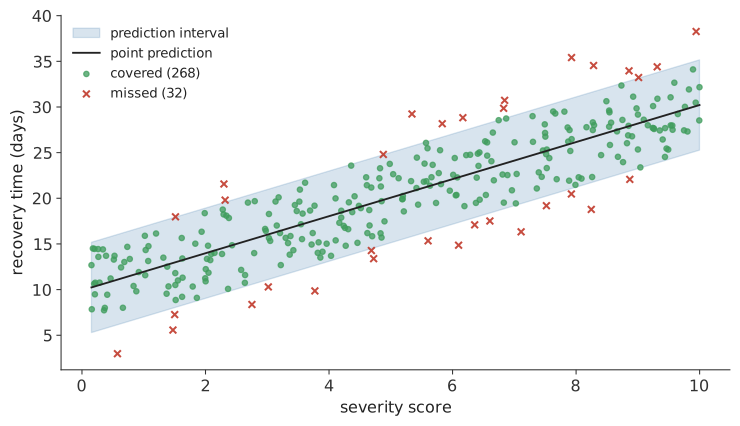
In Figure 1.9, 268 of 300 test outcomes fall inside their intervals. Empirical coverage is 89.3%. A finite test sample need not produce exactly 90% coverage.

Figure 1.10: Empirical coverage across 400 repeated experiments, each using a freshly drawn calibration and test set.

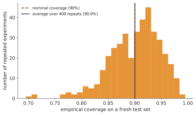
Figure 1.10 shows 400 repetitions with new calibration and test samples. Coverage varies across repetitions because both samples are finite. Its average is close to 90%.

The guarantee concerns the marginal behavior of the procedure over repeated calibration and test observations. It does not assign a 90% posterior probability to one reported interval. For a fixed interval and observed outcome, the outcome is either covered or missed.

1.9 Exchangeability

The coverage guarantee requires the calibration observations and the new observation to be exchangeable.

Figure 1.11: Nine observations shown in their original order, and in one arbitrary shuffled order.

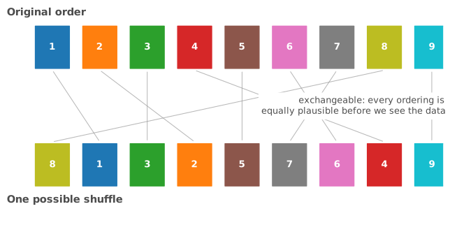
Data are exchangeable when their joint distribution does not change after reordering. Figure 1.11 represents this as a shuffle. Independent observations drawn from the same distribution are exchangeable, although exchangeability is a weaker condition than independence.

Exchangeability can fail when calibration data and future observations come from different populations or data-collection processes.

Figure 1.12: A calibration population and a deployment population with different severity score distributions.

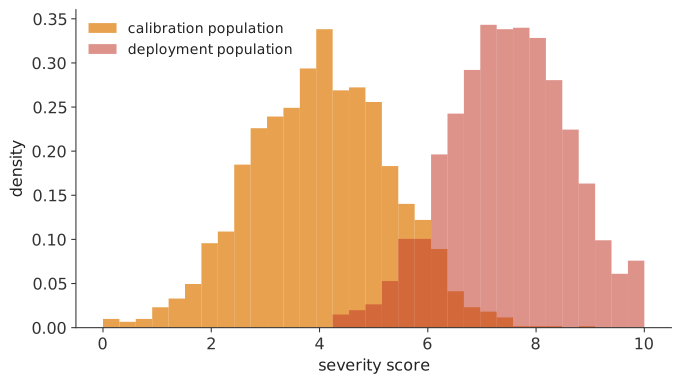
In Figure 1.12, the deployment patients have higher severity scores than the calibration patients. Standard split conformal coverage does not apply automatically because the two samples are not exchangeable. Study design, sampling, time, site, eligibility criteria, and measurement procedures should be checked before relying on the coverage guarantee.

1.10 Marginal versus conditional coverage

Standard split conformal prediction controls coverage averaged over the target population. It does not guarantee the same coverage at every predictor value or within every subgroup.

Figure 1.13: Overall coverage close to the 90% target, built from two groups whose individual coverage is very different.

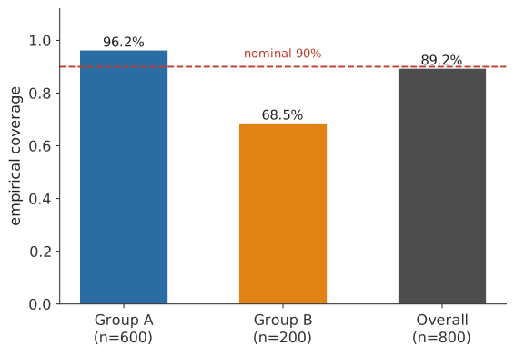
In Figure 1.13, Group A has 96.2% coverage and Group B has 68.5% coverage. Pooled coverage is 89.2%. The overall estimate hides the low coverage in Group B.

Marginal coverage averages over the target population. Conditional coverage refers to coverage at particular predictor values or within defined groups. Subgroup estimates can reveal heterogeneity, but standard split conformal prediction does not guarantee them. Group-conditional methods address selected, pre-specified groups later in this chapter.

1.11 Coverage is not enough

Coverage can be increased by making every interval very wide, but the resulting intervals may provide little information.

Figure 1.14: A trivially wide interval and a properly calibrated interval, both containing enough test observations to look valid on coverage alone.

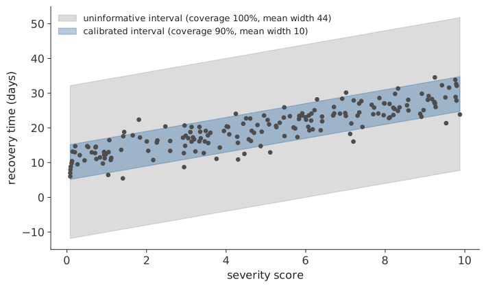
In Figure 1.14, the gray band covers every test outcome but has mean width 44. The blue band reaches 90% coverage with mean width 10. Coverage should therefore be reported with interval width or prediction-set size.

Validity concerns coverage. Efficiency concerns how narrow the intervals or how small the prediction sets are. Both should be evaluated.

1.12 Homoscedastic versus heteroscedastic data

A constant-width interval may work when outcome variability is similar across the predictor space, called homoscedasticity. When variability changes with the predictors, the data are heteroscedastic and a constant width may be inefficient or poorly balanced across regions.

Figure 1.15: One constant interval width applied to data whose true variability grows with severity.

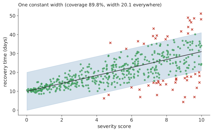
In Figure 1.15, outcome variability increases with severity. The constant-width interval is unnecessarily wide at low severity and too narrow at high severity. Overall coverage is 89.8%, but coverage is uneven across the predictor range.

1.13 Conformalized quantile regression

Conformalized quantile regression (CQR) allows interval width to vary with the predictors.

CQR first estimates lower and upper conditional quantiles. It then uses held-out calibration scores to adjust both bounds. Under exchangeability, this adjustment provides marginal coverage while retaining widths that vary across observations. It does not guarantee conditional coverage.

Figure 1.16: An adaptive interval on the same heteroscedastic data, its width growing with severity.

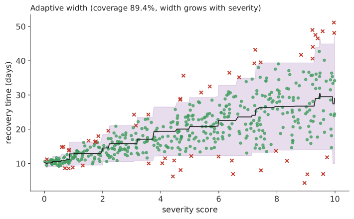
In Figure 1.16, the interval widens with severity and has 89.4% overall coverage. CQR is not always narrower than a constant-width interval. Its benefit depends on how well the quantile models learn changes in the outcome distribution.

1.14 Classification methods

Conformal classification returns a set of retained classes. LAC, APS, and RAPS use different scores to construct that set.

1.14.1 LAC

LAC uses the score \(1-\hat\pi_y(x)\), where \(\hat\pi_y(x)\) is the fitted probability of candidate class \(y\). A class with high fitted probability has a small score.

Figure 1.17: LAC applied to the opening classification example. Classes with probability above the calibrated threshold are retained.

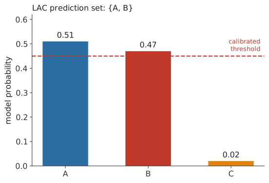
In Figure 1.17, the equivalent probability threshold is 0.45. Classes A and B exceed it and C does not, so the set is \(\{A,B\}\). LAC can return a singleton, several classes, or an empty set, depending on the calibrated cutoff and fitted probabilities.

1.14.2 APS

Adaptive prediction sets (APS) use the ranked class probabilities and their cumulative sum.

Figure 1.18: APS applied to a four-class example. Classes are added, most likely first, until the cumulative probability clears a calibrated threshold.

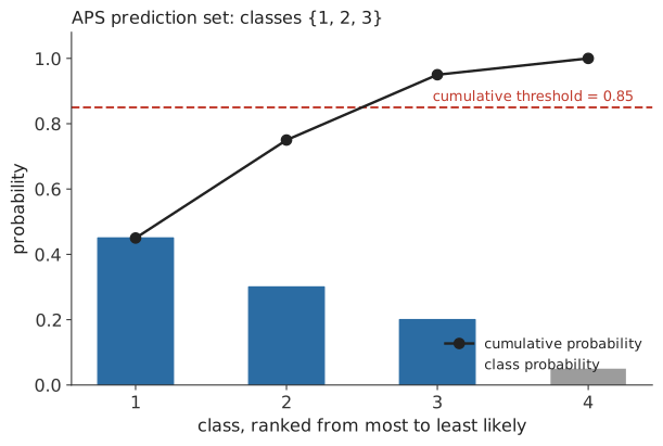
In Figure 1.18, the ranked probabilities are 0.45, 0.30, 0.20, and 0.05. Their cumulative values are 0.45, 0.75, 0.95, and 1.00. The cumulative total first exceeds the illustrated threshold of 0.85 after the third class, so the set is \(\{1,2,3\}\). APS tends to return smaller sets when probability is concentrated and larger sets when it is spread across classes.

1.14.3 RAPS

With many classes, APS can include a long tail of classes with small individual probabilities. RAPS adds a penalty based on class rank to discourage large sets.

Figure 1.19: APS and RAPS applied to the same fifteen-class probability vector. RAPS penalizes travelling far down the ranked list, producing a smaller set.

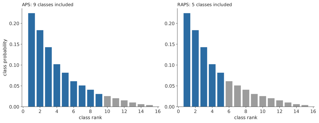
In Figure 1.19, APS retains nine classes and RAPS retains five. RAPS does not always produce smaller sets. Its result depends on the regularization settings, calibration data, and probability distribution.

1.14.4 Prediction-set size

Set size should be examined across the test sample, not only for one observation.

Figure 1.20: Prediction set sizes across many test observations, from a five-class conformal classifier at 90% target coverage.

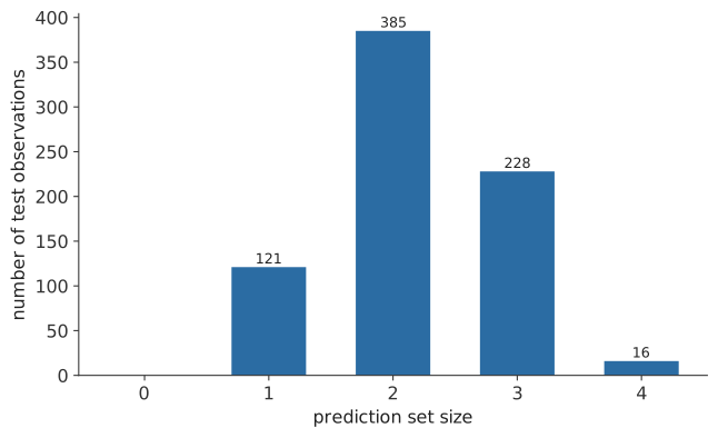
Figure 1.20 shows APS set sizes in a five-class example with a 90% target. Most sets contain two classes. Some contain one or three, and a few contain four. Report the distribution together with mean set size and the fractions of empty and singleton sets.

1.15 Mondrian and group-conditional conformal prediction

Mondrian, or group-conditional, conformal prediction calibrates separately within pre-defined groups. It can provide group-specific coverage under suitable exchangeability assumptions within each group.

Figure 1.21: Calibration observations available overall, and within three individual hospitals.

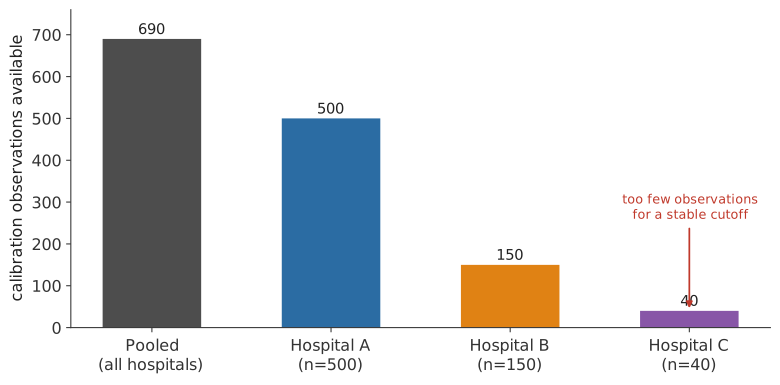
In Figure 1.21, each hospital receives its own cutoff. Hospital A has 500 calibration observations, while Hospital C has 40. The cutoff for Hospital C will have coarser rank resolution and greater sampling variability. Finer groups leave fewer calibration observations in each group.

The guarantee applies to the chosen groups, not to every predictor value or unexamined subgroup. Groups should be selected before final evaluation and must contain enough calibration observations for the target error rate.

1.16 Split conformal, full conformal, Jackknife+ and CV+

Split conformal prediction fits one model and uses a separate calibration sample. Other constructions use the available data differently.

Figure 1.22: The split conformal workflow: one model fit, one calibration pass.

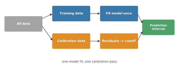
Figure 1.22 shows one model fit followed by one calibration step.

Full conformal prediction considers candidate outcomes one at a time. For each candidate, it augments the data, refits the model, and compares scores symmetrically across observations. This can require many model fits for every new prediction.

Jackknife+ fits \(n\) leave-one-out models. Each observation supplies an out-of-sample residual, and each fitted model predicts the new observation.

Figure 1.23: The Jackknife+ workflow: one model refit per left-out observation, combined into a single interval.

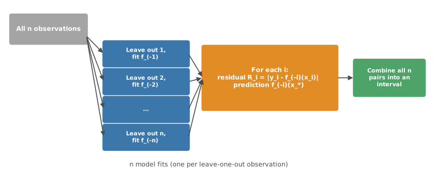
Figure 1.23 shows how the \(n\) residuals and \(n\) predictions are combined into one interval. This construction differs from repeating split conformal without a fixed split.

CV+ uses \(K\) folds instead of \(n\) leave-one-out fits.

Figure 1.24: The CV+ workflow: K model fits, one per fold, combined into a single interval.

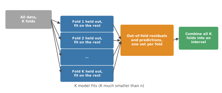
In Figure 1.24, each held-out fold supplies out-of-fold residuals and its fitted model predicts the new observation.

Method	Data usage	Model fits	Computational cost	Main advantage	Main limitation
Split conformal	One training/calibration split	1	Low	Simple and fast	Reserves data for calibration alone
Full conformal	Every observation, repeatedly	Many, per candidate outcome	Very high	No fixed calibration split	Usually impractical beyond small problems
Jackknife+	Every observation, leave-one-out	\(n\)	High	Avoids a fixed, possibly unlucky split	Expensive when \(n\) is large
CV+	Every observation, in \(K\) folds	\(K\)	Moderate	Most of Jackknife+’s benefit, far fewer fits	Some sensitivity to the choice of \(K\)

Split conformal is usually the simplest starting point. Jackknife+ and CV+ use the data more fully but require more computation. Full conformal is often impractical outside small or specialized problems.

1.17 Distribution shift and time series

Time ordering, dependence, and population change can invalidate the exchangeability assumption used by standard split conformal prediction.

Figure 1.25: A static conformal interval, calibrated before a change in the underlying process, fails after that change, while an interval that adapts over time recovers.

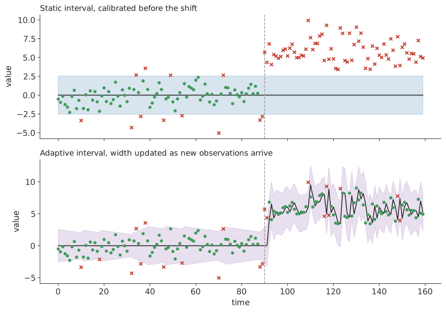
In Figure 1.25, the process level changes after calibration. The static interval covers 86.7% of observations before the change and none afterward. An adaptive interval widens after repeated misses and recovers some coverage, at the cost of greater width.

Covariate shift changes the predictor distribution while retaining the conditional outcome distribution. Concept drift changes the relationship between predictors and outcome. Time dependence makes nearby observations dependent and their ordering informative.

Weighted conformal prediction adjusts calibration scores using estimated or known density ratios under covariate shift. Rolling calibration uses recent observations and discards older ones. EnbPI and Adaptive Conformal Inference (ACI) update intervals using recent prediction errors. These methods address different forms of shift or dependence.

Their guarantees differ from ordinary split conformal coverage and require additional assumptions. A standard exchangeable-data guarantee should not be reported when known shift or dependence violates its conditions.

1.18 When conformal prediction is useful

Conformal prediction is useful when:

• a fitted model needs prediction intervals or prediction sets
• a parametric error distribution is difficult to justify
• a pre-specified marginal error rate is meaningful
• calibration observations and future observations can reasonably be treated as exchangeable

1.19 When conformal prediction is less suitable

Conformal prediction is less suitable when:

• too few observations remain for stable calibration
• calibration and deployment populations differ substantially
• dependence or time ordering is ignored
• the requirement is coverage for every individual or every subgroup
• rare classes or groups have too few calibration observations

A weak base model often produces wide intervals or large prediction sets. Conformal calibration controls coverage under its assumptions, but it does not make the underlying predictions more accurate.