4 Exercises with health survey data
4.1 Data and setup
This exercise uses the 2011–2012 National Health and Nutrition Examination Survey (NHANES). The teaching data contain demographics, body measurements, and spirometry results for 4,214 adults with complete values for the variables used below.
The outcome is FEV1, the volume of air exhaled in the first second of a spirometry test, measured in milliliters. The predictors are age, sex, standing height, weight, and the family income-to-poverty ratio. Smoking history and diagnosed lung disease are not included, so important predictors of lung function are missing. race_ethnicity, NHANES’s recorded race and Hispanic origin category, is withheld from the model and used only to examine subgroup coverage.
Download the file used throughout this chapter:
- nhanes_fev1.csv, the 4,214 rows used here, with a fixed
splitcolumn
Place it in a data folder beside your script or notebook so that the paths in the examples work unchanged.
NHANES uses a complex, multistage sample with clustering, unequal selection probabilities, and survey weights. The simplified file omits the weights, strata, sampling units, spirometry quality grades, and participants with missing values. Its row-wise split is useful for learning the conformal workflow, but it does not support a population-representative or clinical coverage claim. A research analysis would need to address the NHANES sample design, use the appropriate design variables and weights, define acceptable spirometry quality grades, and choose a split that respects relevant dependence.
4.2 1. Inspect the data and the study design
Load the data and answer these questions:
- What are the training, calibration, and test sample sizes?
- What is the center, spread, and shape of the FEV1 distribution?
- Which race and Hispanic origin groups will have imprecise test-set coverage estimates?
- Why does the
splitcolumn alone not establish exchangeability?
import pandas as pd

nhanes = pd.read_csv("data/nhanes_fev1.csv")
print(nhanes.shape)
print(nhanes["fev1_ml"].describe().round(2))
print("skewness:", round(nhanes["fev1_ml"].skew(), 4))
print(nhanes.groupby("split").size())
print(nhanes["race_ethnicity"].value_counts())
(4214, 8)
count 4214.00
mean 3064.91
std 915.39
min 409.00
25% 2398.25
50% 2989.50
75% 3671.50
max 6923.00
Name: fev1_ml, dtype: float64
skewness: 0.3224
split
cal 843
test 843
train 2528
dtype: int64
race_ethnicity
Non-Hispanic White 1493
Non-Hispanic Black 1149
Non-Hispanic Asian 585
Mexican American 429
Other Hispanic 428
Other/Multiracial 130
Name: count, dtype: int64nhanes <- read.csv("data/nhanes_fev1.csv")
cat(dim(nhanes), "\n")
cat("mean:", round(mean(nhanes$fev1_ml), 2), " sd:", round(sd(nhanes$fev1_ml), 2), "\n")
cat("range:", range(nhanes$fev1_ml), "\n")
table(nhanes$split)
sort(table(nhanes$race_ethnicity), decreasing = TRUE)4214 8
mean: 3064.91 sd: 915.39
range: 409 6923
cal test train
843 843 2528
Non-Hispanic White Non-Hispanic Black Non-Hispanic Asian Mexican American
1493 1149 585 429
Other Hispanic Other/Multiracial
428 130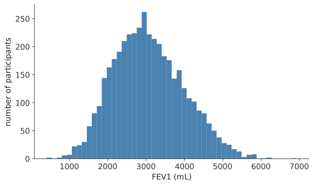
Figure 4.1 shows a mildly right-skewed distribution centered near 3,000 mL. Other/Multiracial is the smallest group, with 130 participants overall and only 19 in the test set. Its coverage estimate will be imprecise. The split column records where each row was assigned, but it contains no information about the NHANES sampling clusters or whether this sample resembles a future target population.
4.3 2. Create the subsets and fit a base model
Use the existing split and fit the stated XGBoost model. Encode sex, but keep race_ethnicity out of the model. Report test R² and mean absolute error (MAE). The model and its settings are fixed before the test results are examined.
import xgboost as xgb
from sklearn.metrics import r2_score, mean_absolute_error

nhanes_enc = pd.get_dummies(nhanes, columns=["sex"], drop_first=True)
model_feature_cols = [c for c in nhanes_enc.columns if c not in ("fev1_ml", "split", "race_ethnicity")]

train = nhanes_enc[nhanes_enc.split == "train"].reset_index(drop=True)
cal = nhanes_enc[nhanes_enc.split == "cal"].reset_index(drop=True)
test = nhanes_enc[nhanes_enc.split == "test"].reset_index(drop=True)

reg = xgb.XGBRegressor(n_estimators=400, max_depth=4, learning_rate=0.05, random_state=0)
reg.fit(train[model_feature_cols], train["fev1_ml"])
pred_test = reg.predict(test[model_feature_cols])
print("test R2:", round(r2_score(test["fev1_ml"], pred_test), 4))
print("test MAE:", round(mean_absolute_error(test["fev1_ml"], pred_test), 1))
test R2: 0.6679
test MAE: 417.5library(xgboost)
library(fastDummies)
nhanes_enc <- dummy_cols(nhanes, select_columns = "sex",
remove_first_dummy = TRUE, remove_selected_columns = TRUE)
model_feature_cols <- setdiff(names(nhanes_enc), c("fev1_ml", "split", "race_ethnicity"))
train <- nhanes_enc[nhanes_enc$split == "train", ]
cal <- nhanes_enc[nhanes_enc$split == "cal", ]
test <- nhanes_enc[nhanes_enc$split == "test", ]
dtrain <- xgb.DMatrix(data = as.matrix(train[, model_feature_cols]), label = train$fev1_ml)
reg <- xgb.train(params = list(max_depth = 4, eta = 0.05, objective = "reg:squarederror"),
data = dtrain, nrounds = 400)
pred_test <- predict(reg, as.matrix(test[, model_feature_cols]))
r2 <- 1 - sum((test$fev1_ml - pred_test)^2) / sum((test$fev1_ml - mean(test$fev1_ml))^2)
cat("test R2:", round(r2, 4), "\n")
cat("test MAE:", round(mean(abs(test$fev1_ml - pred_test)), 1), "\n")test R2: 0.6679
test MAE: 417.5R and Python give the same results because they fit the same model to the same rows. R² is 0.67 and MAE is about 418 mL. These measures describe point-prediction performance. They do not show whether a prediction interval has the requested coverage.
4.4 3. Build a split conformal interval
Use a conformal package to build a 90% prediction interval. Report the number and proportion of covered test outcomes, a 95% Wilson interval for the coverage proportion, and mean interval width.
from mapie.regression import SplitConformalRegressor
from mapie.metrics.regression import regression_coverage_score, regression_mean_width_score
from scipy.stats import binomtest

alpha = 0.10
scr = SplitConformalRegressor(estimator=reg, confidence_level=1 - alpha,
                               conformity_score="absolute", prefit=True)
scr.conformalize(cal[model_feature_cols], cal["fev1_ml"])
pred_test, y_pis = scr.predict_interval(test[model_feature_cols])
lo, hi = y_pis[:, 0, 0], y_pis[:, 1, 0]

coverage = regression_coverage_score(test["fev1_ml"].to_numpy(), y_pis)[0]
width = regression_mean_width_score(y_pis)[0]
covered = (test["fev1_ml"].to_numpy() >= lo) & (test["fev1_ml"].to_numpy() <= hi)
ci = binomtest(int(covered.sum()), len(covered)).proportion_ci(method="wilson")
print("covered:", covered.sum(), "of", len(covered))
print("empirical coverage:", round(coverage, 4))
print("95% Wilson CI:", round(ci.low, 4), "to", round(ci.high, 4))
print("mean interval width:", round(width, 1))
covered: 758 of 843
empirical coverage: 0.8992
95% Wilson CI: 0.8770 to 0.9177
mean interval width: 1696.3library(workflows)
library(parsnip)
library(probably)
xgb_spec <- boost_tree(trees = 400, tree_depth = 4, learn_rate = 0.05) |>
set_engine("xgboost") |> set_mode("regression")
f <- as.formula(paste("fev1_ml ~", paste(model_feature_cols, collapse = " + ")))
xgb_wflow <- workflow() |> add_model(xgb_spec) |> add_formula(f)
xgb_fit <- fit(xgb_wflow, data = train)
alpha <- 0.10
split_conf <- int_conformal_split(xgb_fit, cal)
pred_probably <- predict(split_conf, test, level = 1 - alpha)
lo <- pred_probably$.pred_lower
hi <- pred_probably$.pred_upper
covered <- (test$fev1_ml >= lo) & (test$fev1_ml <= hi)
ci <- prop.test(sum(covered), length(covered), correct = FALSE)$conf.int
cat("covered:", sum(covered), "of", length(covered), "\n")
cat("empirical coverage:", round(mean(covered), 4), "\n")
cat("95% score CI:", round(ci[1], 4), "to", round(ci[2], 4), "\n")
cat("mean interval width:", round(mean(hi - lo), 1), "\n")covered: 758 of 843
empirical coverage: 0.8992
95% score CI: 0.8770 to 0.9177
mean interval width: 1696.3The test estimate is 89.9%, with a 95% interval from 87.7% to 91.8%. It is compatible with the 90% target. This one test set cannot verify the distribution-free guarantee. Every interval has width 1,696 mL, regardless of participant characteristics.
4.5 4. Investigate subgroup coverage
Calculate coverage and group size for height quartiles and for race_ethnicity. Identify clear patterns, but separate large differences supported by adequate sample sizes from noisy estimates in small groups.
height_bins = pd.qcut(test["height_cm"], 4)
diag = pd.DataFrame({"height_bin": height_bins, "covered": covered, "width": hi - lo})
print(diag.groupby("height_bin", observed=True).agg(
    n=("covered", "size"), coverage=("covered", "mean"), mean_width=("width", "mean")).round(4))
n coverage mean_width
height_bin
(139.299, 160.8] 215 0.9860 1696.2627
(160.8, 168.4] 208 0.9615 1696.2627
(168.4, 175.6] 210 0.8524 1696.2627
(175.6, 199.5] 210 0.7952 1696.2627test_eth = nhanes[nhanes.split == "test"].reset_index(drop=True)["race_ethnicity"]
eth_df = pd.DataFrame({"race_ethnicity": test_eth, "covered": covered})
by_eth = eth_df.groupby("race_ethnicity").agg(n=("covered", "size"), coverage=("covered", "mean"))
print(by_eth.sort_values("coverage").round(4)) n coverage
race_ethnicity
Other/Multiracial 19 0.8421
Non-Hispanic Black 225 0.8667
Non-Hispanic White 322 0.8851
Non-Hispanic Asian 123 0.9431
Other Hispanic 75 0.9467
Mexican American 79 0.9494height_bins <- cut(test$height_cm, breaks = quantile(test$height_cm, probs = seq(0, 1, 0.25)),
include.lowest = TRUE)
diag_df <- data.frame(height_bin = height_bins, covered = covered, width = hi - lo)
diag_df |> dplyr::group_by(height_bin) |>
dplyr::summarise(n = dplyr::n(), coverage = mean(covered), mean_width = mean(width))# A tibble: 4 x 4
height_bin n coverage mean_width
<fct> <int> <dbl> <dbl>
1 [139,161] 215 0.986 1696.
2 (161,168] 208 0.962 1696.
3 (168,176] 210 0.852 1696.
4 (176,200] 210 0.795 1696.test_eth <- nhanes[nhanes$split == "test", "race_ethnicity"]
eth_df <- data.frame(race_ethnicity = test_eth, covered = covered)
eth_df |> dplyr::group_by(race_ethnicity) |>
dplyr::summarise(n = dplyr::n(), coverage = mean(covered)) |> dplyr::arrange(coverage)# A tibble: 6 x 3
race_ethnicity n coverage
<chr> <int> <dbl>
1 Other/Multiracial 19 0.842
2 Non-Hispanic Black 225 0.867
3 Non-Hispanic White 322 0.885
4 Non-Hispanic Asian 123 0.943
5 Other Hispanic 75 0.947
6 Mexican American 79 0.949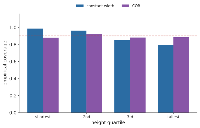
Coverage falls steadily with height, from 98.6% in the shortest quartile to 79.5% in the tallest. Each group has about 210 test observations, and every interval has the same width. This is strong evidence that the constant-width interval does not adapt to the changing error distribution across height.
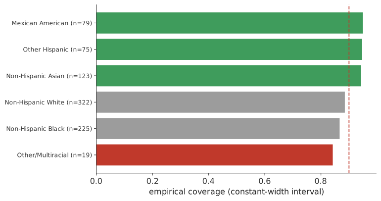
The race and Hispanic origin estimates range from 84.2% to 94.9%. Their precision differs greatly. Other/Multiracial has only 19 test participants. Its 84.2% estimate has a 95% Wilson interval from 62.4% to 94.5%. Non-Hispanic Black has 225 test participants, and its 86.7% estimate has an interval from 81.6% to 90.5%. These results identify patterns to investigate, but they do not establish each group’s population coverage.
race_ethnicity was not used as a model feature. Differences can still appear because prediction errors may vary across groups. A pooled conformal cutoff controls marginal coverage, not coverage within every group.
4.6 5. Apply an adaptive method
Fit conformalized quantile regression (CQR). Compare its overall coverage, mean width, height-quartile coverage, and race and Hispanic origin estimates with the constant-width interval.
from sklearn.ensemble import GradientBoostingRegressor
from mapie.regression import ConformalizedQuantileRegressor

gbr = GradientBoostingRegressor(loss="quantile", alpha=0.5, n_estimators=400,
                                 max_depth=3, learning_rate=0.05, random_state=0)
cqr = ConformalizedQuantileRegressor(estimator=gbr, confidence_level=1 - alpha, prefit=False)
cqr.fit(train[model_feature_cols], train["fev1_ml"])
cqr.conformalize(cal[model_feature_cols], cal["fev1_ml"])
_, cqr_intervals = cqr.predict_interval(test[model_feature_cols])
cqr_lo, cqr_hi = cqr_intervals[:, 0, 0], cqr_intervals[:, 1, 0]
cqr_coverage = regression_coverage_score(test["fev1_ml"].to_numpy(), cqr_intervals)[0]
cqr_width = regression_mean_width_score(cqr_intervals)[0]
print("CQR empirical coverage:", round(cqr_coverage, 4))
print("CQR mean interval width:", round(cqr_width, 1))
CQR empirical coverage: 0.8921
CQR mean interval width: 1672.0MAPIE reports The predictions are ill-sorted. for this fit. One test observation has a point prediction below its lower quantile estimate. The lower and upper interval bounds do not cross. This warning should be checked rather than ignored when it appears.
cqr_covered = (test["fev1_ml"].to_numpy() >= cqr_lo) & (test["fev1_ml"].to_numpy() <= cqr_hi)
cqr_diag = pd.DataFrame({"height_bin": height_bins, "covered": cqr_covered, "width": cqr_hi - cqr_lo})
print(cqr_diag.groupby("height_bin", observed=True).agg(
    n=("covered", "size"), coverage=("covered", "mean"), mean_width=("width", "mean")).round(4))

cqr_eth_df = pd.DataFrame({"race_ethnicity": test_eth, "covered": cqr_covered})
print(cqr_eth_df.groupby("race_ethnicity").agg(
    n=("covered", "size"), coverage=("covered", "mean")).sort_values("coverage").round(4))
n coverage mean_width
height_bin
(139.299, 160.8] 215 0.8791 1248.0813
(160.8, 168.4] 208 0.9231 1553.5423
(168.4, 175.6] 210 0.8810 1799.3420
(175.6, 199.5] 210 0.8857 2096.0564
n coverage
race_ethnicity
Other/Multiracial 19 0.7368
Other Hispanic 75 0.8800
Non-Hispanic Black 225 0.8889
Mexican American 79 0.8987
Non-Hispanic White 322 0.9006
Non-Hispanic Asian 123 0.9024probably::int_conformal_quantile() is used here as in chapter 2, with the same caveat that it fits its own internal quantregForest model rather than using the workflow’s XGBoost engine for the quantile bounds.
library(dplyr)

set.seed(1)
qc <- int_conformal_quantile(xgb_fit, train_data = train, cal_data = cal, level = 1 - alpha)
pred_qc <- predict(qc, test)
qc_covered <- (test$fev1_ml >= pred_qc$.pred_lower) & (test$fev1_ml <= pred_qc$.pred_upper)
cat("CQR (probably) empirical coverage:", round(mean(qc_covered), 4), "\n")
cat("CQR (probably) mean interval width:",
    round(mean(pred_qc$.pred_upper - pred_qc$.pred_lower), 1), "\n")
CQR (probably) empirical coverage: 0.8909
CQR (probably) mean interval width: 1623.2qc_diag <- data.frame(height_bin = height_bins, covered = qc_covered,
width = pred_qc$.pred_upper - pred_qc$.pred_lower)
qc_diag |> dplyr::group_by(height_bin) |>
dplyr::summarise(n = dplyr::n(), coverage = mean(covered), mean_width = mean(width))
qc_eth_df <- data.frame(race_ethnicity = test_eth, covered = qc_covered)
qc_eth_df |> dplyr::group_by(race_ethnicity) |>
dplyr::summarise(n = dplyr::n(), coverage = mean(covered)) |> dplyr::arrange(coverage)# A tibble: 4 x 4
height_bin n coverage mean_width
<fct> <int> <dbl> <dbl>
1 [139,161] 215 0.907 1314.
2 (161,168] 208 0.889 1450.
3 (168,176] 210 0.852 1722.
4 (176,200] 210 0.914 2012.
# A tibble: 6 x 3
race_ethnicity n coverage
<chr> <int> <dbl>
1 Other/Multiracial 19 0.842
2 Other Hispanic 75 0.867
3 Non-Hispanic Asian 123 0.886
4 Non-Hispanic White 322 0.888
5 Non-Hispanic Black 225 0.889
6 Mexican American 79 0.949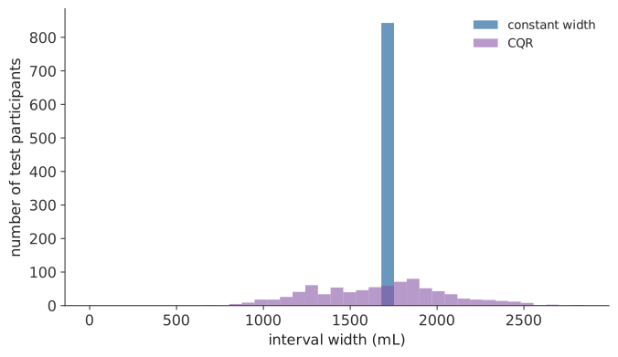
CQR produces wider intervals for taller participants in both languages. Height-quartile coverage is more even than with the constant-width interval, although no quartile is guaranteed 90% coverage. The Python and R results differ because they use different quantile models.
The race and Hispanic origin estimates do not show the same consistent improvement. The Other/Multiracial estimate is based on 19 cases and changes in different directions in Python and R. That instability is a reason to collect more evaluation data, not evidence that one implementation is better for this group. CQR can adapt to patterns learned from its predictors, but it still guarantees only marginal coverage.
4.7 6. Interpret the results
Answer the following without additional code.
- Why is 89.9% overall coverage insufficient when the research question requires reliable intervals across height groups?
- Why does CQR improve the height pattern without guaranteeing improvement for race and Hispanic origin groups?
- Would adding
race_ethnicityas a predictor necessarily solve the subgroup problem? What evidence would be needed? - Would you deploy any of these intervals if 90% coverage were required for every reported subgroup? State what you would change or check first.
- Marginal coverage averages across different parts of the population. It can be near 90% while some height groups are overcovered and others are undercovered.
- CQR changes interval width using patterns learned from the model features. This may help across height because height is a predictor, but CQR retains a marginal guarantee and does not ensure coverage for any subgroup.
- Adding a variable can change the errors but cannot guarantee group-conditional coverage. The choice also needs scientific and ethical justification. Evaluate the final, pre-specified procedure on adequate held-out data for every group that matters.
- None of these results supports a 90% guarantee for every group. A stronger study would retain NHANES design information, define the target population, use a dependence-aware split, pre-specify groups, ensure adequate calibration and test sizes, and consider a suitable group-conditional method.
4.8 An optional classification extension: Palmer Penguins
The source Palmer Penguins data contain 344 penguins. The teaching file contains the 342 rows with complete values for bill length, bill depth, flipper length, and body mass. Fit LAC and APS prediction sets at 90% target coverage. Compare coverage, mean set size, and the fraction of empty sets. Then explain why 72 test penguins are not enough for a precise comparison of the two methods.
Download penguins.csv and place it in the same data folder as the NHANES file.
import numpy as np
from sklearn.linear_model import LogisticRegression
from sklearn.pipeline import make_pipeline
from sklearn.preprocessing import StandardScaler
from mapie.classification import SplitConformalClassifier

pen = pd.read_csv("data/penguins.csv")
feat = ["bill_length_mm", "bill_depth_mm", "flipper_length_mm", "body_mass_g"]
train_p = pen[pen.split == "train"].reset_index(drop=True)
cal_p = pen[pen.split == "cal"].reset_index(drop=True)
test_p = pen[pen.split == "test"].reset_index(drop=True)

clf = make_pipeline(StandardScaler(), LogisticRegression(max_iter=2000))
clf.fit(train_p[feat], train_p["y"])
print("test accuracy:", round((clf.predict(test_p[feat]) == test_p["y"]).mean(), 4))

for score in ["lac", "aps"]:
    scc = SplitConformalClassifier(estimator=clf, confidence_level=0.90,
                                    conformity_score=score, prefit=True, random_state=0)
    scc.conformalize(cal_p[feat], cal_p["y"])
    _, sets = scc.predict_set(test_p[feat])
    m = sets[:, :, 0]
    sizes = m.sum(axis=1)
    covered = m[np.arange(len(test_p)), test_p["y"].to_numpy()]
    print(f"{score.upper()}: covered={covered.sum()}/{len(covered)}  coverage={covered.mean():.4f}  "
          f"mean size={sizes.mean():.4f}  "
          f"empty frac={np.mean(sizes==0):.4f}")
test accuracy: 0.9861
LAC: covered=61/72 coverage=0.8472 mean size=0.8472 empty frac=0.1528
APS: covered=72/72 coverage=1.0000 mean size=1.1528 empty frac=0.0000library(predictset)
pen <- read.csv("data/penguins.csv")
feat <- c("bill_length_mm", "bill_depth_mm", "flipper_length_mm", "body_mass_g")
pen$species <- factor(pen$species)
trainval <- pen[pen$split %in% c("train", "cal"), ]
test <- pen[pen$split == "test", ]
glm_clf <- make_model(
train_fun = function(x, y) nnet::multinom(y ~ ., data = data.frame(y = y, x),
trace = FALSE, maxit = 2000),
predict_fun = function(object, x_new) predict(object, newdata = as.data.frame(x_new),
type = "probs"),
type = "classification"
)
for (meth in c("lac", "aps")) {
fit_fn <- switch(meth, lac = conformal_lac, aps = conformal_aps)
res <- fit_fn(trainval[, feat], trainval$species, model = glm_clf, x_new = test[, feat],
alpha = 0.10, cal_fraction = 0.35, seed = 1)
n_covered <- sum(mapply(function(set, y) as.character(y) %in% set,
res$sets, test$species))
cat(sprintf("%s: covered=%d/%d coverage=%.4f mean size=%.4f empty frac=%.4f\n",
toupper(meth), n_covered, nrow(test), coverage(res, test$species),
mean(set_size(res)), mean(set_size(res) == 0)))
}LAC: covered=69/72 coverage=0.9583 mean size=1.0000 empty frac=0.0000
APS: covered=69/72 coverage=0.9583 mean size=1.0000 empty frac=0.0000The Python and R results are not a package benchmark. They use different fitted models and different calibration splits. Python LAC covers 61 of 72 test labels. Its 95% Wilson interval runs from 74.7% to 91.2%. R covers 69 of 72, with an interval from 88.5% to 98.6%. The intervals are wide and overlap. A larger, fixed evaluation design is needed before comparing the methods.