3 Math behind spectral clustering, from first principles
3.1 From a similarity matrix to one coordinate
Suppose we have four observations,
\[A,\;B,\;C,\;D.\]
Assume we have already constructed a symmetric, nonnegative similarity matrix
\[W= \begin{pmatrix} 0 & 0.90 & 0.80 & 0.05\\ 0.90 & 0 & 0.85 & 0.03\\ 0.80 & 0.85 & 0 & 0.04\\ 0.05 & 0.03 & 0.04 & 0 \end{pmatrix}.\]
The interpretation is straightforward:
\[W_{ij} = \text{similarity between observations }i\text{ and }j.\]
For example,
\[W_{AB}=0.90\]
means that \(A\) and \(B\) are strongly connected, while
\[W_{AD}=0.05\]
means that \(A\) and \(D\) are only weakly connected.
Looking at this tiny matrix, a human can already see a pattern:
\[A,B,C\]
are tightly connected, while \(D\) is much more weakly connected to them.
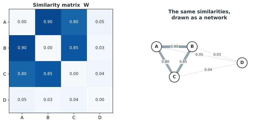
But for a large graph, perhaps containing thousands of observations, we need a mathematical way to extract this structure.
It is tempting to jump directly from this pattern to cluster labels. That would skip the central step of spectral clustering. Before asking
Which cluster is each observation in?
we ask a softer question that connects the matrix to those eventual labels:
Can we place the observations on a line so that strong connections become short distances?
This is the one-dimensional version of the spectral representation shown in the intuition chapter. Once we understand one coordinate, several coordinates will follow naturally.
3.1.1 Positions to be learned from the graph
Let \(f_A\) denote the position of \(A\) on this new line, and define \(f_B\), \(f_C\), and \(f_D\) in the same way:
\[A\rightarrow f_A,\]
\[B\rightarrow f_B,\]
\[C\rightarrow f_C,\]
\[D\rightarrow f_D.\]
These positions are not additional measurements such as gene expression or age. Nor are they arbitrary numbers that we choose by hand. They are unknowns whose values will be learned from the similarities in \(W\).
To see what \(W\) asks of them, start with a strong connection such as
\[W_{AB}=0.90.\]
Because \(A\) and \(B\) are strongly connected, their new positions should be close:
\[f_A\approx f_B.\]
The same reasoning applied to
\[W_{AC}=0.80\]
says that \(f_A\approx f_C\). By contrast,
\[W_{AD}=0.05\]
is so small that the graph gives us much less reason to keep \(f_A\) and \(f_D\) together.
Thus the coordinate should obey the principle
\[\boxed{ W_{ij}\text{ large} \quad\Longrightarrow\quad f_i\approx f_j }\]
while
\[\boxed{ W_{ij}\text{ small} \quad\Longrightarrow\quad f_i\text{ and }f_j\text{ may differ substantially.} }\]
This is the conceptual basis of the spectral embedding. We have not yet chosen any coordinates; we have only stated what a good set of coordinates must accomplish.
For the algebra, collect the four unknown positions into a vector:
\[\boxed{ f= \begin{pmatrix} f_A\\ f_B\\ f_C\\ f_D \end{pmatrix} }\]
At this point \(f\) is a candidate arrangement of the graph on a line. Finding the candidate that best satisfies the requirement above is the optimization problem we are about to build.
3.1.2 How to read a coordinate vector
Each entry \(f_i\) is the position of observation \(i\) on the newly learned axis. For example, a useful coordinate might have the schematic form
\[f= \begin{pmatrix} 0.50\\ 0.48\\ 0.52\\ -1.50 \end{pmatrix}.\]
The values here are illustrative rather than the normalized solution we will calculate later. What matters is the arrangement: \(A,B,C\) are close together and \(D\) is far away.
The numerical value \(0.50\) has no direct biological or physical meaning, it isn’t a gene-expression value or a probability. What matters is the relative geometry:
\[f_A\approx f_B\approx f_C,\]
while
\[f_D\]
is very different.
In short,
\[\boxed{ f_i=\text{position of observation }i\text{ on a graph-derived coordinate axis.} }\]
The word graph-derived is important: the coordinate is new, but its values are determined by the observed similarities. We can now make that dependence precise by giving the graph a way to score any candidate \(f\).
3.2 The objective
The requirement is qualitative; optimization needs a number. We build that number first for one edge, then for the graph as a whole.
3.2.1 Scoring one pair
Consider one pair of observations \(i\) and \(j\). Their separation on the new axis is
\[ f_i-f_j. \]
Squaring it gives us the size of that separation:
\[ (f_i-f_j)^2. \]
But this alone is not enough.
If we used only \((f_i-f_j)^2\), we would be saying that every pair of observations is equally important. We would try to keep \(i\) and \(j\) close even if they were barely related in the original data.
That is not what we want.
Remember that \(W_{ij}\) tells us how strongly observations \(i\) and \(j\) are connected.
- If \(W_{ij}\) is large, \(i\) and \(j\) are very similar. We care a lot if the new coordinates pull them apart.
- If \(W_{ij}\) is small, they are only weakly related. Their separation matters much less.
- If \(W_{ij}=0\), there is no edge between them. We do not directly care how far apart they end up.
So we weight the separation by the strength of the connection:
\[ \boxed{ W_{ij}(f_i-f_j)^2 } \]
Now the quantity has the meaning we actually want:
How badly did our new coordinate system separate two observations that were supposed to stay together?
So \((f_i-f_j)^2\) tells us how far apart the pair became, while \(W_{ij}\) tells us how much we should care about that separation.
For example:
Strong connection, similar coordinates.
Suppose
\[W_{ij}=0.90,\]
and
\[f_i=0.50,\qquad f_j=0.52.\]
Then
\[(f_i-f_j)^2=(-0.02)^2=0.0004,\]
so the penalty is
\[0.90\times0.0004=0.00036.\]
That penalty is tiny, exactly what we want.
Strong connection, very different coordinates.
Suppose instead
\[W_{ij}=0.90,\]
but
\[f_i=0.50,\qquad f_j=-2.\]
Then
\[(f_i-f_j)^2=(2.5)^2=6.25,\]
and the penalty becomes
\[0.90\times6.25=5.625.\]
That penalty is large, exactly what we want to avoid.
Weak connection, very different coordinates.
Now suppose
\[W_{ij}=0.05\]
while the same coordinate difference remains:
\[(f_i-f_j)^2=6.25.\]
Then the penalty is only
\[0.05\times6.25=0.3125.\]
The graph is much more tolerant of separating observations that are only weakly connected. These three checks all point in the same direction: \(W_{ij}(f_i-f_j)^2\) is small for an arrangement the edge supports and large for one that pulls a strong edge apart.
3.2.2 From one pair to the whole graph
We need to judge the coordinate vector \(f\) over the entire graph, not only for one pair. The natural move is to sum the same penalty over all pairs:
\[\sum_{i,j}W_{ij}(f_i-f_j)^2.\]
For an undirected graph,
\[W_{ij}=W_{ji},\]
so the pair \((i,j)\) is counted once as \((i,j)\) and again as \((j,i)\).
So we divide by \(2\):
\[\boxed{ \frac12\sum_{i,j}W_{ij}(f_i-f_j)^2. }\]
This quantity is small when strongly connected observations get similar coordinates, and large when they get very different ones.
So our first version of the learning problem is:
\[\boxed{ \text{Find }f_1,\ldots,f_n \text{ such that } \frac12\sum_{i,j}W_{ij}(f_i-f_j)^2 \text{ is small.} }\]
At this point the objective already says everything we want. What it lacks is a convenient matrix form for optimization. Rewriting the sum will reveal that matrix rather than asking us to accept it in advance.
3.3 The Laplacian
Start from the objective we wanted:
\[\frac12\sum_{i,j}W_{ij}(f_i-f_j)^2.\]
We now simplify it algebraically.
3.3.1 Expand the squared difference
Use
\[(a-b)^2=a^2-2ab+b^2.\]
Applying that here,
\[(f_i-f_j)^2 = f_i^2-2f_if_j+f_j^2.\]
Substitute into the objective:
\[\frac12\sum_{i,j} W_{ij} \left( f_i^2-2f_if_j+f_j^2 \right).\]
Distribute the summation:
\[= \frac12\sum_{i,j}W_{ij}f_i^2 - \sum_{i,j}W_{ij}f_if_j + \frac12\sum_{i,j}W_{ij}f_j^2.\]
We now have three terms.
3.3.2 Simplify the first term
Consider
\[\frac12\sum_{i,j}W_{ij}f_i^2.\]
For a fixed \(i\), the number \(f_i^2\) doesn’t depend on \(j\), so
\[\frac12\sum_{i,j}W_{ij}f_i^2 = \frac12\sum_i f_i^2 \sum_jW_{ij}.\]
This naturally introduces the quantity
\[d_i=\sum_jW_{ij}.\]
The number \(d_i\) is called the degree of node \(i\) in a weighted graph, simply the total strength of all edges leaving it. So
\[\frac12\sum_{i,j}W_{ij}f_i^2 = \frac12\sum_i d_if_i^2.\]
The degree didn’t appear because we decided beforehand that graphs should have a degree matrix, it fell out automatically because the row sum
\[\sum_jW_{ij}\]
is present in the algebra.
3.3.3 Simplify the third term
Now consider
\[\frac12\sum_{i,j}W_{ij}f_j^2.\]
Because the graph is undirected,
\[W_{ij}=W_{ji}.\]
So this term gives the same quantity as the first:
\[\frac12\sum_jd_jf_j^2.\]
The symbols \(i\) and \(j\) are dummy summation indices, so we can write
\[\frac12\sum_i d_if_i^2.\]
Add that to the first term and together they become
\[\sum_i d_if_i^2.\]
Our objective is now
\[\sum_i d_if_i^2-\sum_{i,j}W_{ij}f_if_j.\]
3.3.4 The degree matrix \(D\)
Define
\[D= \begin{pmatrix} d_1&0&\cdots&0\\ 0&d_2&\cdots&0\\ \vdots&&\ddots&\vdots\\ 0&0&\cdots&d_n \end{pmatrix}.\]
\(D\) is diagonal because it stores one number per node, its total connectivity, not pairwise relationships.
Now multiply \(D\) by \(f\):
\[Df= \begin{pmatrix} d_1f_1\\ d_2f_2\\ \vdots\\ d_nf_n \end{pmatrix}.\]
Then multiply from the left by \(f^T\):
\[f^TDf = \begin{pmatrix} f_1&f_2&\cdots&f_n \end{pmatrix} \begin{pmatrix} d_1f_1\\ d_2f_2\\ \vdots\\ d_nf_n \end{pmatrix}.\]
Multiplying this out gives
\[f^TDf = d_1f_1^2+d_2f_2^2+\cdots+d_nf_n^2.\]
So, compactly,
\[\boxed{ f^TDf=\sum_i d_if_i^2. }\]
So the first part of our objective can be written compactly as \(f^TDf\).
3.3.5 The second term as \(f^TWf\)
The remaining term is
\[\sum_{i,j}W_{ij}f_if_j.\]
First examine
\[Wf.\]
Its \(i\)th element is
\[(Wf)_i=\sum_jW_{ij}f_j.\]
Now multiply by \(f^T\):
\[f^TWf = \sum_i f_i(Wf)_i.\]
Substitute the expression for \((Wf)_i\):
\[f^TWf = \sum_i f_i\left(\sum_jW_{ij}f_j\right).\]
Which is just
\[f^TWf = \sum_{i,j}W_{ij}f_if_j.\]
In short,
\[\boxed{ f^TWf=\sum_{i,j}W_{ij}f_if_j. }\]
3.3.6 Put the two pieces together
We had
\[\frac12\sum_{i,j}W_{ij}(f_i-f_j)^2 = \sum_i d_if_i^2 - \sum_{i,j}W_{ij}f_if_j.\]
Using the matrix forms derived above,
\[= f^TDf-f^TWf.\]
Factor out \(f^T\) on the left and \(f\) on the right:
\[= f^T(D-W)f.\]
Putting it all together,
\[\boxed{ \frac12\sum_{i,j}W_{ij}(f_i-f_j)^2 = f^T(D-W)f. }\]
Now, and only now, define
\[\boxed{ L=D-W. }\]
This matrix is called the unnormalized graph Laplacian, and it lets us write
\[\boxed{ f^TLf = \frac12\sum_{i,j}W_{ij}(f_i-f_j)^2. }\]
This is the central identity of the chapter.
The logical order is important:
We want strongly connected nodes to receive similar coordinates.
For one pair we penalize
\[W_{ij}(f_i-f_j)^2.\]
We sum over all pairs:
\[\frac12\sum_{i,j}W_{ij}(f_i-f_j)^2.\]
Algebra shows that this equals
\[f^T(D-W)f.\]
We therefore call
\[D-W\]
the graph Laplacian.
So \(L=D-W\) is not the starting idea. It is the matrix that naturally encodes the objective we wanted.
The central identity gives us two complementary ways to read the Laplacian. The first describes the graph as a whole; the second describes what \(L\) does at one node.
3.4 Two ways to read the Laplacian
3.4.1 The whole-graph view: \(f^TLf\) as roughness
We now know that
\[f^TLf = \frac12\sum_{i,j}W_{ij}(f_i-f_j)^2.\]
So \(f^TLf\) measures the total weighted disagreement of \(f\) across the graph, small when strongly connected nodes have similar coordinates, large when some of them don’t. In short,
\[\boxed{ f^TLf=\text{graph roughness, or total weighted disagreement of }f. }\]
A common term is that \(f\) is smooth on the graph when \(f^TLf\) is small.
3.4.2 \(L\) as a neighbor-difference operator
We have already seen that
\[ f^TLf \]
gives us one number measuring how well a complete set of coordinates \(f\) respects the graph.
But what does \(L\) itself actually do?
A useful way to understand it is to look at just one node.
Suppose node \(i\) has coordinate \(f_i\) on our new axis.
Imagine it is connected to three neighbors:
- node \(j\) with coordinate \(f_j\)
- node \(k\) with coordinate \(f_k\)
- node \(m\) with coordinate \(f_m\)
For each neighbor, we can ask:
How different is node \(i\) from this neighbor on the new axis?
Those differences are
\[ f_i-f_j, \]
\[ f_i-f_k, \]
and
\[ f_i-f_m. \]
But, just as before, not every connection is equally important. The graph tells us the strength of each connection through \(W\).
So we weight each difference:
\[ W_{ij}(f_i-f_j), \]
\[ W_{ik}(f_i-f_k), \]
and
\[ W_{im}(f_i-f_m). \]
Then we add them:
\[ W_{ij}(f_i-f_j) + W_{ik}(f_i-f_k) + W_{im}(f_i-f_m). \]
For a general node \(i\), this becomes
\[ \boxed{ (Lf)_i=\sum_j W_{ij}(f_i-f_j) } \]
This is the main idea.
The \(i\)th value of \(Lf\) tells us how different node \(i\) is from its neighbors, taking the strength of each connection into account.
3.4.2.1 A small example
Suppose node A has new coordinate
\[ f_A=2 \]
and it is connected to two nodes:
\[ f_B=3, \qquad f_C=8. \]
Suppose the graph says
\[ W_{AB}=1 \]
and
\[ W_{AC}=0.1. \]
Then for node A,
\[ (Lf)_A = 1(2-3)+0.1(2-8). \]
So
\[ (Lf)_A = -1-0.6 = -1.6. \]
Notice what happened.
A and B differ by only \(1\), but their connection is strong, so that difference contributes fully:
\[ 1(2-3)=-1. \]
A and C differ by \(6\), but their connection is weak, so that large difference contributes only
\[ 0.1(2-8)=-0.6. \]
Again, \(W\) tells us which differences matter strongly and which differences matter only a little.
So \(L\) acts like a neighbor-difference operator.
For every node it asks:
How different is this node’s coordinate from the coordinates of the nodes it is strongly connected to?
3.5 Choosing the smoothest useful coordinate
Our goal was to find graph-derived coordinates that respect strong similarities.
Since
\[f^TLf\]
measures weighted disagreement, a natural objective is
\[\min_f f^TLf.\]
But this immediately creates two related problems: the scale of \(f\) is unconstrained, and a coordinate with no variation is perfectly smooth.
3.5.1 The trivial collapse
Take
\[f= \begin{pmatrix} 0\\ 0\\ \vdots\\ 0 \end{pmatrix}.\]
Then every difference is zero, \(f_i-f_j=0\), so
\[f^TLf=0.\]
That is the smallest possible value, but it tells us nothing.
In fact, any constant vector also gives zero disagreement. For example,
\[f= \begin{pmatrix} 5\\ 5\\ 5\\ 5 \end{pmatrix}\]
also gives
\[f^TLf=0.\]
The smoothest possible coordinate is therefore a useless one that places everyone at the same location. We will deal with these two degeneracies in order. First we fix the scale; then the best remaining constant solution will show us why the first informative coordinate needs one more constraint.
3.5.2 First fix the scale
If a nonconstant candidate is multiplied by a small number, all of its pairwise differences, and therefore its cost, shrink toward zero. To make candidate coordinates comparable and exclude the zero vector, require
\[\boxed{ f^Tf=1. }\]
This means
\[f_1^2+f_2^2+\cdots+f_n^2=1.\]
The coordinate vector now has fixed length. This removes arbitrary rescaling, but it does not yet remove the normalized constant vector. We will encounter that vector as the first solution and then move beyond it.
Our optimization becomes
\[\boxed{ \min_f f^TLf \qquad \text{subject to} \qquad f^Tf=1. }\]
This has the same structural form as the constrained optimization used in PCA.
3.5.3 Why an eigenvalue problem appears
We now solve
\[\min_f f^TLf\]
subject to
\[f^Tf=1.\]
Introduce a Lagrange multiplier \(\lambda\):
\[\mathcal{J}(f,\lambda) = f^TLf - \lambda(f^Tf-1).\]
The role of the multiplier is simply to allow us to optimize the objective while enforcing the unit-length constraint.
Differentiate with respect to \(f\).
Because \(L\) is symmetric,
\[\frac{\partial}{\partial f}(f^TLf)=2Lf.\]
Also,
\[\frac{\partial}{\partial f}(f^Tf)=2f.\]
Putting the two derivatives together,
\[\frac{\partial\mathcal{J}}{\partial f} = 2Lf-2\lambda f.\]
At an optimum, set the derivative equal to zero:
\[2Lf-2\lambda f=0.\]
Divide by \(2\):
\[Lf-\lambda f=0.\]
In other words,
\[\boxed{ Lf=\lambda f. }\]
This is the eigenvalue equation. The derivative calculation tells us that every stationary candidate is an eigenvector. The Rayleigh-quotient argument below will identify which of those candidates is the global minimum.
3.5.4 What the eigenvalue measures
Suppose
\[Lf=\lambda f\]
and
\[f^Tf=1.\]
Multiply the eigenvalue equation from the left by \(f^T\):
\[f^TLf = f^T\lambda f.\]
Because \(\lambda\) is a scalar,
\[f^T\lambda f = \lambda f^Tf.\]
Using the unit-length constraint,
\[f^Tf=1,\]
we obtain
\[\boxed{ f^TLf=\lambda. }\]
But \(f^TLf\) is exactly the total weighted disagreement of \(f\), so
\[\boxed{ \lambda=\text{graph disagreement associated with that eigenvector.} }\]
This identifies the cost of every unit-length eigenvector. To identify which one actually minimizes the cost, it helps to state the same idea for any nonzero vector.
3.5.4.1 The Rayleigh quotient chooses the minimizer
For a nonzero vector \(f\), define the Rayleigh quotient
\[R(f) = \frac{f^TLf}{f^Tf}.\]
Dividing by \(f^Tf\) removes scale: \(f\) and \(cf\) have the same Rayleigh quotient. For the unit-length candidates in our optimization,
\[f^Tf=1,\]
so
\[R(f)=f^TLf.\]
For a symmetric matrix such as \(L\), the smallest possible Rayleigh quotient is its smallest eigenvalue, and it is attained at a corresponding eigenvector. If we restrict the search to vectors orthogonal to that first eigenvector, the smallest possible value becomes \(\lambda_2\); after excluding the first two eigenvectors, it becomes \(\lambda_3\); and so on. Thus the optimization does not merely produce some eigenvector: it orders the eigenvectors by the disagreement they create.
3.5.5 Smallest eigenvalues, not largest
In PCA, an eigenvalue measures variance along a principal direction. We want directions that explain a lot of variance, so the largest eigenvalues are interesting.
In the Laplacian problem, an eigenvalue measures graph roughness:
\[\lambda=f^TLf.\]
We want coordinates that vary as little as possible across strong graph connections, so the smallest eigenvalues are interesting. Put simply:
\[\boxed{ \text{PCA: large eigenvalues are interesting} }\]
while
\[\boxed{ \text{spectral clustering: small Laplacian eigenvalues are interesting.} }\]
This also completes the earlier analogy between a spectral coordinate and a PCA score. In PCA, an observation that originally lives in a \(p\)-dimensional feature space receives a score on PC1, another on PC2, and so on. Four observations might, for example, receive
\[A\rightarrow -2.1,\quad B\rightarrow -1.9,\quad C\rightarrow -2.3,\quad D\rightarrow 4.8\]
on PC1. A spectral coordinate plays the same representational role: its entries locate observations along a learned axis. The criterion that learns the axis is different:
PCA asks which coordinate captures a large amount of variance in the original variables.
Spectral methods ask which coordinate creates little disagreement across strong graph connections.
So
\[\boxed{ \text{PCA score} \longleftrightarrow \text{spectral coordinate} }\]
is a useful analogy, provided we remember that one maximizes variance while the other minimizes graph roughness.
That immediately raises a question: how small can an eigenvalue actually get?
3.5.6 The first solution: a constant coordinate
For now, assume the similarity graph is connected. We will remove that assumption when we reach disconnected components; until then it guarantees that the only zero-cost coordinates are constant across the whole graph.
We diagnosed the constant-coordinate degeneracy before imposing the unit-length constraint. We now use the central identity to prove that its normalized version is the global minimum. The first solution deserves this careful treatment because several later results follow from it.
We have
\[f^TLf = \frac12\sum_{i,j}W_{ij}(f_i-f_j)^2.\]
Every term on the right is nonnegative, since \(W_{ij}\geq0\) and \((f_i-f_j)^2\geq0\), which means
\[\boxed{ f^TLf\geq0 }\]
for every vector \(f\). That’s what it means for \(L\) to be positive semidefinite, and it means every eigenvalue of \(L\) is nonnegative:
\[0\leq\lambda_1\leq\lambda_2\leq\cdots\leq\lambda_n.\]
So the smallest eigenvalue cannot be negative.
Now we only need to show that zero can actually occur.
3.5.6.1 A constant coordinate produces zero disagreement
Take
\[f= \begin{pmatrix} 1\\ 1\\ \vdots\\ 1 \end{pmatrix} =\mathbf{1}.\]
For every pair, \(f_i-f_j=1-1=0\), so
\[\frac12\sum_{i,j}W_{ij}(f_i-f_j)^2=0,\]
which means
\[f^TLf=0.\]
Since values below zero are impossible and zero is achievable,
\[\boxed{ \lambda_1=0. }\]
The reason is extremely concrete:
Giving every node the same coordinate produces absolutely no disagreement across any graph edge.
3.5.6.2 Show directly that the constant vector is an eigenvector
Let’s confirm this directly from the matrix. Let
\[\mathbf{1} = \begin{pmatrix} 1\\ 1\\ \vdots\\ 1 \end{pmatrix}.\]
Recall
\[L=D-W.\]
Then
\[L\mathbf{1} = D\mathbf{1}-W\mathbf{1}.\]
First,
\[D\mathbf{1} = \begin{pmatrix} d_1\\ d_2\\ \vdots\\ d_n \end{pmatrix}.\]
Second, the \(i\)th element of \(W\mathbf{1}\) is
\[\sum_jW_{ij}.\]
But by definition \(\sum_jW_{ij}=d_i\), so
\[W\mathbf{1} = \begin{pmatrix} d_1\\ d_2\\ \vdots\\ d_n \end{pmatrix}.\]
So
\[D\mathbf{1}-W\mathbf{1}=0,\]
which means
\[\boxed{ L\mathbf{1}=0. }\]
Compare with
\[Lv=\lambda v.\]
We have
\[L\mathbf{1}=0\mathbf{1},\]
so \(\mathbf{1}\) is an eigenvector with eigenvalue zero.
3.5.6.3 Normalizing the constant eigenvector
Eigenvectors are conventionally unit length, and \(\mathbf{1}\) is not, yet.
The vector
\[\mathbf{1}\]
has squared length
\[\mathbf{1}^T\mathbf{1}=n.\]
which makes its length
\[\sqrt n.\]
Divide by \(\sqrt n\):
\[\boxed{ v_1 = \frac{1}{\sqrt n} \begin{pmatrix} 1\\ 1\\ \vdots\\ 1 \end{pmatrix}. }\]
The normalization changes the scale, not the fact that every observation gets the same coordinate. Is that coordinate useful for anything?
3.5.6.4 Why the first eigenvector carries no clustering information
Suppose \(n=6\).
Then
\[v_1 = \frac1{\sqrt6} \begin{pmatrix} 1\\1\\1\\1\\1\\1 \end{pmatrix} \approx \begin{pmatrix} 0.408\\ 0.408\\ 0.408\\ 0.408\\ 0.408\\ 0.408 \end{pmatrix}.\]
Remember, each entry of the eigenvector is just the coordinate assigned to one observation, and here every observation gets exactly the same one. There’s no separation to exploit: the first eigenvector is mathematically the smoothest possible coordinate, but it carries no clustering information.
This motivates the next question:
What is the smoothest possible coordinate that is not constant?
That leads to the second eigenvector.
3.5.7 The first informative solution: the second eigenvector
We still want a coordinate with small
\[f^TLf,\]
because we still want strongly connected nodes to have similar values.
But we must prevent the optimizer from simply returning the constant first eigenvector again. As in PCA, a new direction is not allowed to reproduce a direction already found: PC2 is orthogonal to PC1, and the next graph coordinate is orthogonal to \(v_1\). We therefore impose
\[\boxed{ f^Tv_1=0. }\]
This turns the optimization into
\[\boxed{ \min_f f^TLf }\]
subject to
\[f^Tf=1\]
and
\[f^Tv_1=0.\]
Orthogonality enforces a genuinely new direction. Here it also has a particularly simple interpretation.
3.5.7.1 Orthogonality to the constant vector
Because
\[v_1 = \frac1{\sqrt n} \begin{pmatrix} 1\\1\\\vdots\\1 \end{pmatrix},\]
we have
\[f^Tv_1 = \frac1{\sqrt n} (f_1+f_2+\cdots+f_n).\]
The condition
\[f^Tv_1=0\]
therefore implies
\[\boxed{ f_1+f_2+\cdots+f_n=0. }\]
So the new coordinate must balance around zero. It cannot assign the same positive value to everyone.
For example,
\[f= \begin{pmatrix} 0.5\\ 0.4\\ 0.6\\ -0.5\\ -0.4\\ -0.6 \end{pmatrix}\]
has sum zero and is therefore orthogonal to the constant vector.
We established from the Rayleigh quotient that, among vectors orthogonal to \(v_1\), the smallest attainable cost is \(\lambda_2\). The solution to this constrained problem is therefore the eigenvector associated with the second-smallest eigenvalue:
\[\boxed{ v_2. }\]
So \(v_2\) is precisely the smoothest nonconstant coordinate we can get. For a connected graph, it is commonly called the Fiedler vector.
A useful phrase to remember is
\[\boxed{ \text{$v_2$ is the smoothest possible nonconstant signal on the graph.} }\]
Let’s see what that looks like on a concrete graph.
3.6 The four-observation graph
We can now close the four-observation example that opened the chapter. We have every tool needed to follow it from \(W\) through \(D\) and \(L\) to its first informative coordinate, using numbers we can check by hand. Return to
\[W= \begin{pmatrix} 0 & 0.90 & 0.80 & 0.05\\ 0.90 & 0 & 0.85 & 0.03\\ 0.80 & 0.85 & 0 & 0.04\\ 0.05 & 0.03 & 0.04 & 0 \end{pmatrix}.\]
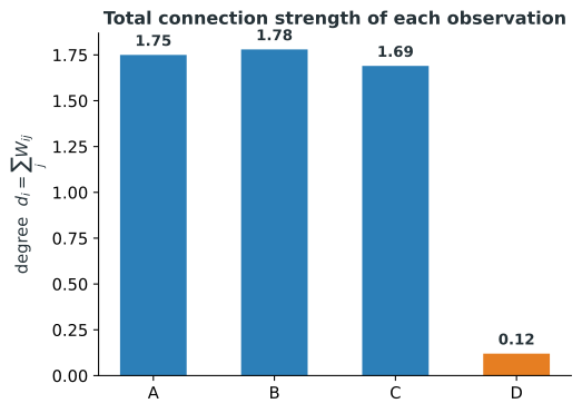
The degrees are
\[d_A=0.90+0.80+0.05=1.75,\]
\[d_B=0.90+0.85+0.03=1.78,\]
\[d_C=0.80+0.85+0.04=1.69,\]
\[d_D=0.05+0.03+0.04=0.12.\]
So
\[D= \begin{pmatrix} 1.75&0&0&0\\ 0&1.78&0&0\\ 0&0&1.69&0\\ 0&0&0&0.12 \end{pmatrix}.\]
Then
\[L=D-W\]
gives
\[L= \begin{pmatrix} 1.75 & -0.90 & -0.80 & -0.05\\ -0.90 & 1.78 & -0.85 & -0.03\\ -0.80 & -0.85 & 1.69 & -0.04\\ -0.05 & -0.03 & -0.04 & 0.12 \end{pmatrix}.\]
The eigenvalues are approximately
\[\lambda_1=0,\]
\[\lambda_2=0.1599,\]
\[\lambda_3=2.5061,\]
\[\lambda_4=2.6740.\]
The first eigenvector is
\[v_1= \begin{pmatrix} 0.5\\ 0.5\\ 0.5\\ 0.5 \end{pmatrix},\]
which is exactly the normalized constant vector because
\[\frac1{\sqrt4}=0.5.\]
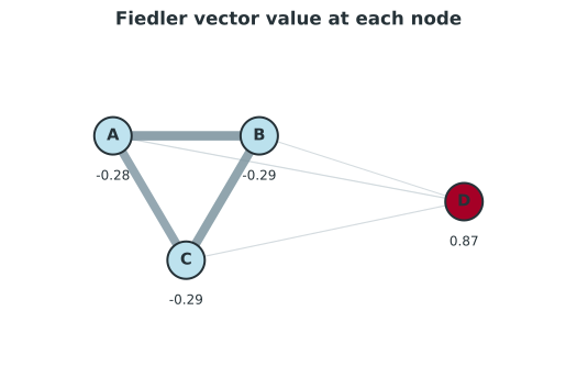
One valid sign choice for the second eigenvector is approximately
\[v_2= \begin{pmatrix} -0.284\\ -0.293\\ -0.289\\ 0.866 \end{pmatrix}.\]
Look at the pattern rather than the exact values:
\[v_2(A)\approx v_2(B)\approx v_2(C),\]
while
\[v_2(D)\]
is very different.
The Fiedler vector has recovered exactly the network structure that was visible by eye in \(W\).
The sign could equally well be reversed:
\[\begin{pmatrix} 0.284\\ 0.293\\ 0.289\\ -0.866 \end{pmatrix}.\]
The interpretation would be identical.
Let’s compare this good choice of \(f\) against a poor one, side by side, using the pairwise-penalty formula from earlier in this chapter.
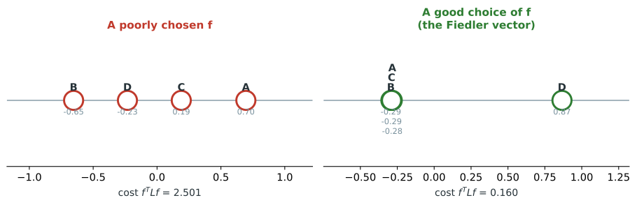
The problem with the poorer coordinate in Figure 3.4 is not that it places the weakly connected pair \(B,D\) close together: weak edges do not repel nodes. Its costly mistake is separating \(A\) from \(C\) even though \(W_{AC}=0.80\) is one of the strongest connections in the graph. Once both candidates obey the same centering and unit-length constraints, the Fiedler vector avoids that expensive disagreement and has a far lower cost.
W <- matrix(c(
  0.00, 0.90, 0.80, 0.05,
  0.90, 0.00, 0.85, 0.03,
  0.80, 0.85, 0.00, 0.04,
  0.05, 0.03, 0.04, 0.00
), nrow = 4, byrow = TRUE,
dimnames = list(c("A","B","C","D"), c("A","B","C","D")))

d <- rowSums(W)
L <- diag(d) - W

eig <- eigen(L, symmetric = TRUE)
ord <- order(eig$values)
round(eig$values[ord], 4)          # eigenvalues, smallest first
v2 <- eig$vectors[, ord][, 2]
round(v2, 4)                        # the Fiedler vector

# both forms of the central identity, and the eigenvalue, agree
round(as.numeric(t(v2) %*% L %*% v2), 6)
round(0.5 * sum(W * outer(v2, v2, "-")^2), 6)
round(eig$values[ord][2], 6)

# L times the constant vector is exactly zero
as.numeric(L %*% rep(1, 4))
[1] 0.0000 0.1599 2.5061 2.6740
[1] -0.2840 -0.2932 -0.2888 0.8660
[1] 0.159894
[1] 0.159894
[1] 0.159894
[1] 0 0 0 0import numpy as np
W = np.array([
[0.00, 0.90, 0.80, 0.05],
[0.90, 0.00, 0.85, 0.03],
[0.80, 0.85, 0.00, 0.04],
[0.05, 0.03, 0.04, 0.00],
])
d = W.sum(axis=1)
L = np.diag(d) - W
eigenvalues, eigenvectors = np.linalg.eigh(L) # ascending order already
print(np.round(eigenvalues, 4))
v2 = eigenvectors[:, 1]
print(np.round(v2, 4))
# both forms of the central identity, and the eigenvalue, agree
print(round(float(v2 @ L @ v2), 6))
print(round(float(0.5 * np.sum(W * (v2[:, None] - v2[None, :])**2)), 6))
print(round(float(eigenvalues[1]), 6))
# L times the constant vector is exactly zero
print(L @ np.ones(4))[0. 0.1599 2.5061 2.674 ]
[-0.284 -0.2932 -0.2888 0.866 ]
0.159894
0.159894
0.159894
[ 0. 0. 0. -0.]The next question is what this same mechanism does when a graph contains two internally strong regions joined by a single weak bridge.
3.7 How \(v_2\) reveals two clusters
Return to the six-node graph from the previous chapter. It contains two strongly connected groups:
\[A,B,C\]
and
\[D,E,F.\]
Inside each group, edge weights are large. Between the groups, edge weights are tiny.
One subtle point now becomes important: weak edges do not push observations apart. The unit-length and orthogonality constraints force a nonconstant coordinate to vary somewhere; minimizing \(f^TLf\) places that unavoidable variation where the graph is weakest.
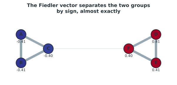
For the six-node graph, consider the unit-length, zero-sum candidate
\[f= \frac{1}{\sqrt6} \begin{pmatrix} 1\\ 1\\ 1\\ -1\\ -1\\ -1 \end{pmatrix}.\]
Its entries are approximately \(+0.408\) on \(A,B,C\) and \(-0.408\) on \(D,E,F\).
Inside the first group.
For \(A\) and \(B\),
\[f_A-f_B=\frac1{\sqrt6}-\frac1{\sqrt6}=0.\]
So
\[W_{AB}(f_A-f_B)^2=0.\]
The same is true for other within-group pairs.
Strong edges contribute essentially no penalty.
Inside the second group.
Again, nodes receive nearly identical values, so strong within-group edges contribute almost no penalty.
Across the weak bridge.
In the running network, the only cross-group edge joins \(C\) and \(F\), with \(W_{CF}=0.05\). Across that edge,
\[f_C-f_F = \frac1{\sqrt6}-\left(-\frac1{\sqrt6}\right) = \frac2{\sqrt6}.\]
Its squared difference is
\[(f_C-f_F)^2=\frac{4}{6}=\frac23.\]
This is a large coordinate difference, but it lies across a weak edge. Its contribution is only
\[0.05\times\frac23\approx0.0333.\]
The coordinate has to vary, and changing sign across this weak bridge costs far less than creating comparable differences along the strong edges inside either triangle.
This explains why the Fiedler vector may naturally take a form resembling
\[\boxed{ (+,+,+,-,-,-). }\]
It keeps strong edges smooth and places most of the change across weakly connected regions.
That is exactly where a good cluster boundary should occur.
3.7.1 Why the sign of \(v_2\) is arbitrary
The sign carries no information: which side is called positive is arbitrary. If
\[Lv_2=\lambda_2v_2,\]
then
\[L(-v_2) = -\lambda_2v_2 = \lambda_2(-v_2).\]
So \(-v_2\) is an equally valid eigenvector.
So
\[(+,+,+,-,-,-)\]
and
\[(-,-,-,+,+,+)\]
represent the same separation.
What matters is the relative placement of observations, not which side is positive.
This is analogous to the arbitrary sign of PCA loadings and scores.
3.8 Disconnected components and multiple zero eigenvalues
The Fiedler vector put almost all of its change across the six-node graph’s weak bridge. Now imagine gradually reducing that same bridge weight from \(0.05\) to zero. In the limiting case the two groups are not joined at all, and “almost no cost” becomes exactly zero. This limiting case is one of the deepest reasons spectral clustering works.
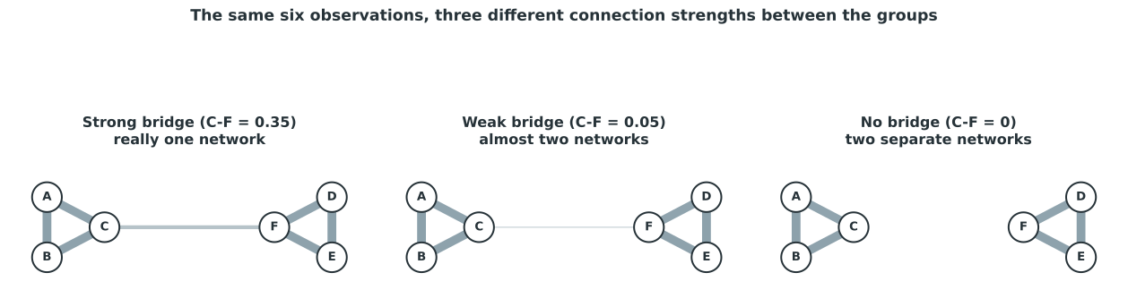
Suppose the graph contains two completely disconnected components:
\[A,B,C\]
and
\[D,E,F.\]
There are no edges at all between the groups, so for every cross-group pair,
\[W_{ij}=0.\]
Now construct
\[z_1= \begin{pmatrix} 1\\ 1\\ 1\\ 0\\ 0\\ 0 \end{pmatrix}.\]
Within the first component, all coordinates are equal, so every difference is zero, and the same is true within the second component, where every coordinate is already zero. Across the two components the coordinate changes from \(1\) to \(0\), but the corresponding edge weights are zero, so every term
\[W_{ij}(z_{1i}-z_{1j})^2\]
is zero too, which means
\[z_1^TLz_1=0.\]
Similarly, define
\[z_2= \begin{pmatrix} 0\\ 0\\ 0\\ 1\\ 1\\ 1 \end{pmatrix}.\]
Again,
\[z_2^TLz_2=0.\]
So there are at least two independent zero-energy directions:
\[\boxed{ \lambda_1=\lambda_2=0. }\]
The general argument below will show that there cannot be a third one for a graph with exactly these two connected components, so the multiplicity is exactly two.
3.8.1 General result
If a graph has \(k\) connected components, then
\[\boxed{ \text{multiplicity of eigenvalue }0=k. }\]
For every component \(C_r\), define an indicator vector
\[(z_r)_i= \begin{cases} 1, & i\in C_r,\\ 0, & i\notin C_r. \end{cases}\]
Each indicator vector is constant within its component, and there are no edges connecting that component to the others, so
\[Lz_r=0.\]
These indicator vectors are linearly independent, so the nullspace has at least \(k\) dimensions. To see why it has exactly \(k\), take any vector \(f\) satisfying \(Lf=0\). Then
\[0=f^TLf=\frac12\sum_{i,j}W_{ij}(f_i-f_j)^2.\]
Every term is nonnegative, so the sum can be zero only if \(f_i=f_j\) along every positive-weight edge. Following paths through the graph shows that \(f\) must be constant within each connected component. Such a vector is completely determined by one constant per component, so there can be no more than \(k\) independent zero-eigenvalue directions. Together with the \(k\) indicator vectors, this proves the result.
3.8.2 Implications for clustering
Imagine the ideal clustering problem in which clusters are completely disconnected from one another.
If there are three clusters, the Laplacian would have
\[\lambda_1=\lambda_2=\lambda_3=0,\]
and then
\[\lambda_4>0.\]
The low-eigenvalue eigenspace would exactly encode the cluster indicator structure.
Spectral clustering can therefore be understood as extending this perfect disconnected-components result to realistic graphs in which clusters are only approximately disconnected.
The argument is complete without computation, but a direct numerical check on the small network is available below.
W <- as.matrix(read.csv("data/six-node-network-disconnected.csv",
                         row.names = 1, check.names = FALSE))
d <- rowSums(W)
L <- diag(d) - W
vals <- sort(eigen(L, symmetric = TRUE, only.values = TRUE)$values)
round(vals, 4)
sum(vals < 1e-8)
[1] 0.0000 0.0000 2.5864 2.5864 2.6736 2.6736
[1] 2import numpy as np
import pandas as pd
W = pd.read_csv("data/six-node-network-disconnected.csv", index_col=0).to_numpy()
d = W.sum(axis=1)
L = np.diag(d) - W
vals = np.sort(np.linalg.eigvalsh(L))
print(np.round(vals, 4))
print((vals < 1e-8).sum())[-0. -0. 2.5864 2.5864 2.6736 2.6736]
2Two disconnected triangles, two zero eigenvalues, exactly as claimed. The calculation confirms the structural result; it is not standing in for the proof.
3.9 Real data: clusters are almost disconnected, not perfectly disconnected
Real datasets usually contain some weak connections between clusters.
Instead of exact eigenvalues such as
\[0,\;0,\;0,\;0.8,\ldots,\]
we may observe
\[0,\;0.01,\;0.03,\;0.72,\ldots.\]
The second and third eigenvalues are no longer exactly zero, because the corresponding groups are not perfectly separated.
But they remain small.
That means there are coordinates that are almost constant inside groups and change mainly across weak boundaries.
This gives an extremely useful interpretation:
\[\boxed{ \text{A spectral cluster is approximately an almost-disconnected component of the graph.} }\]
Is there a single number measuring how close to disconnected a graph is? Yes: \(\lambda_2\).
3.9.1 Algebraic connectivity
For a connected graph,
\[\lambda_1=0\]
but
\[\lambda_2>0.\]
If \(\lambda_2\) is very small, there is a nonconstant vector that achieves very little graph disagreement. This is possible when the graph can nearly be divided into two pieces connected only by weak edges.
So
\[\lambda_2\approx0\]
suggests an almost-disconnected structure.
If \(\lambda_2\) is larger, any nonconstant coordinate must create substantial disagreement across strong edges. The graph is therefore harder to split into separate communities.
For this reason,
\[\boxed{ \lambda_2 }\]
is called the algebraic connectivity of the graph.
It measures, in a spectral sense, how difficult it is to separate the graph.
\(\lambda_2\) gives the smoothest relaxed two-way coordinate under the unnormalized constraint. Before extending that idea to several coordinates, we need to ask whether every node should count equally when graph degrees differ sharply.
3.10 Normalizing for degree
The unnormalized Laplacian gave us the central mechanism: measure disagreement, fix the scale, and find the smoothest independent coordinates. Its scale constraint, \(f^Tf=1\), gives every node equal weight. That choice is reasonable when degrees are similar, but it can distort the question when some nodes carry far more of the graph’s total connection strength than others.
3.10.1 Why degree matters
Go back to the four-observation example one more time.
\[W= \begin{pmatrix} 0 & 0.90 & 0.80 & 0.05\\ 0.90 & 0 & 0.85 & 0.03\\ 0.80 & 0.85 & 0 & 0.04\\ 0.05 & 0.03 & 0.04 & 0 \end{pmatrix}, \qquad d_A=1.75,\quad d_B=1.78,\quad d_C=1.69,\quad d_D=0.12.\]
Here \(D\) is the label of the fourth observation. Later, a standalone \(D\) in expressions such as \(f^TDf\) denotes the diagonal degree matrix; subscripts such as \(d_D\) and \(f_D\) still refer to the observation.
Consider the connection between \(A\) and \(D\): \(W_{AD}=0.05\). On its own, that number looks small. The important question is what it is small relative to.
From \(A\)’s point of view, its total connectivity is \(d_A=1.75\), almost all of it tied up in strong relationships with \(B\) and \(C\). The connection to \(D\) is
\[\frac{W_{AD}}{d_A}=\frac{0.05}{1.75}\approx0.029,\]
less than three percent of everything \(A\) is connected to. It is a minor part of \(A\)’s neighborhood.
Now look at the same edge from \(D\)’s side. \(D\)’s total connectivity is only \(d_D=0.12\), and essentially none of it goes anywhere except back to \(A\), \(B\), and \(C\). The very same connection is
\[\frac{W_{AD}}{d_D}=\frac{0.05}{0.12}\approx0.417,\]
almost forty-two percent of everything \(D\) is connected to. The same raw edge is a small fraction of \(A\)’s connections and a large fraction of \(D\)’s.
\[\boxed{ \text{The same raw weight } W_{ij} \text{ can be almost irrelevant to node } i \text{ and almost everything to node } j. }\]
The unnormalized energy, \(\frac12\sum_{i,j}W_{ij}(f_i-f_j)^2\), weights this edge by the raw value \(0.05\). It does not judge a proposed separation relative to the total connectivity on either side. Normalization adds that missing comparison.
3.10.2 A random-walk view
To make “relative to this node’s own connectivity” precise, imagine standing at a node and taking one random step to a neighbor, choosing each neighbor in proportion to the connection strength. The probability of stepping from node \(i\) to node \(j\) is
\[\boxed{ P_{ij}=\frac{W_{ij}}{d_i}. }\]
This definition assumes \(d_i>0\); isolated nodes must be removed or handled separately. Collect the probabilities into a matrix \(P\), one row per starting node. Because \(\sum_j W_{ij}=d_i\), each row of \(P\) sums to \(1\). Dividing by degree has turned connection strengths into transition probabilities.
W <- matrix(c(
  0.00, 0.90, 0.80, 0.05,
  0.90, 0.00, 0.85, 0.03,
  0.80, 0.85, 0.00, 0.04,
  0.05, 0.03, 0.04, 0.00
), nrow = 4, byrow = TRUE,
dimnames = list(c("A","B","C","D"), c("A","B","C","D")))
d <- rowSums(W)
P <- diag(1 / d) %*% W
round(P, 4)
rowSums(P)
A B C D
A 0.0000 0.5143 0.4571 0.0286
B 0.5056 0.0000 0.4775 0.0169
C 0.4734 0.5030 0.0000 0.0237
D 0.4167 0.2500 0.3333 0.0000
[1] 1 1 1 1import numpy as np
W = np.array([
[0.00, 0.90, 0.80, 0.05],
[0.90, 0.00, 0.85, 0.03],
[0.80, 0.85, 0.00, 0.04],
[0.05, 0.03, 0.04, 0.00],
])
d = W.sum(axis=1)
P = np.diag(1 / d) @ W
print(np.round(P, 4))
print(P.sum(axis=1))[[0. 0.5143 0.4571 0.0286]
[0.5056 0. 0.4775 0.0169]
[0.4734 0.503 0. 0.0237]
[0.4167 0.25 0.3333 0. ]]
[1. 1. 1. 1.]Read row \(D\): [0.4167, 0.25, 0.3333, 0]. Every step from \(D\) lands on \(A\), \(B\), or \(C\). In other words, \(D\) is weakly connected in absolute terms, but it is not a region in which this random walk can remain. Row \(A\), [0, 0.5143, 0.4571, 0.0286], tells the opposite story: a walker at \(A\) moves almost always to \(B\) or \(C\) and has only about a 3% chance of stepping directly to \(D\). The transition matrix makes the degree asymmetry explicit.
3.10.2.1 Staying inside a region
The six-node network from the intuition chapter shows the cluster interpretation more clearly. Its two three-node groups have the same total connection strength, and they are joined by one weak bridge.
W6 <- as.matrix(read.csv("data/six-node-network.csv", row.names = 1, check.names = FALSE))
d6 <- rowSums(W6)
P6 <- diag(1 / d6) %*% W6
round(P6["C", ], 4)
A B C D E F
0.4775 0.4944 0.0000 0.0000 0.0000 0.0281import pandas as pd
W6 = pd.read_csv("data/six-node-network.csv", index_col=0).to_numpy()
d6 = W6.sum(axis=1)
P6 = np.diag(1 / d6) @ W6
print(np.round(P6[2], 4)) # row C[0.4775 0.4944 0. 0. 0. 0.0281]A random walker standing at \(C\) has about a 97% chance of stepping to \(A\) or \(B\), and only a 3% chance of crossing the weak bridge to \(F\). Thus a crossing is unlikely on the next step from this boundary node. To decide whether the whole set \(\{A,B,C\}\) tends to retain the walk, however, we must also account for starts at \(A\) and \(B\). A useful graph cluster is a region in which movement is mostly internal and escape across the boundary is rare.
This gives the earlier smooth-coordinate picture an equivalent probabilistic reading:
\[\boxed{ \text{A cluster is a region a random walk on the graph tends to stay inside of for a long time.} }\]
3.10.3 From node degree to graph volume
The random-walk picture has brought us to two questions. How large is a region of a weighted graph, and how often does the walk escape from it? Counting nodes is not enough: three weakly connected nodes and three strongly connected nodes should not necessarily have the same importance. We therefore begin with degree, extend it from one node to a set, and then use it to measure escape.
For one node, we already have that measure. Its degree is
\[ d_i=\sum_j W_{ij}, \]
the total connection strength attached to it.
Write \(V\) for the full set of nodes. For any subset \(S\subseteq V\), add the degrees of the nodes it contains:
\[\boxed{ \operatorname{vol}(S)=\sum_{i\in S}d_i. }\]
This quantity is called the volume of (S). It is not the number of nodes in the set, and it is not a physical volume. It measures how much total connection strength is attached to the nodes in (S).
An internal edge contributes to the volume twice, once through the degree of each endpoint. An edge from \(S\) to the rest of the graph contributes once, through its endpoint in \(S\). Thus a larger volume means that more connection strength—and, as we will soon see, more stationary random-walk probability—is associated with the set.
The four-observation graph makes the distinction concrete. Its degrees are
\[ d_A=1.75,\qquad d_B=1.78,\qquad d_C=1.69,\qquad d_D=0.12. \]
Therefore
\[ \operatorname{vol}(\{A,B,C\}) = 1.75+1.78+1.69 = 5.22, \]
which can also be read directly from the edges:
\[ \operatorname{vol}(\{A,B,C\}) = 2(0.90+0.80+0.85) +(0.05+0.03+0.04) =5.22. \]
The first group contains edges internal to \(\{A,B,C\}\), so their weights are counted twice. The second contains edges from that set to \(D\), so their weights are counted once.
The same double counting gives a useful identity for the whole graph. In the zero-diagonal similarity graphs used here, every edge joins two different nodes, and its weight enters the degree of both endpoints. Therefore
\[ \operatorname{vol}(V) = 2\sum_{i<j}W_{ij}. \]
By comparison, the singleton set has volume
\[ \operatorname{vol}(\{D\})=0.12. \]
The total volume of the graph is
\[ \operatorname{vol}(V) = \sum_i d_i = 5.22+0.12 = 5.34. \]
Node (D) is one of the four nodes, but it carries only
\[ \frac{0.12}{5.34}\approx0.022 \]
of the graph’s total volume. Counting nodes would give (D) one quarter of the graph. Counting volume gives it a little over two percent. Degree normalization uses the second view.
3.10.3.1 Volume and the stationary distribution
Volume appears naturally in the random walk. Define
\[\boxed{ \pi_i=\frac{d_i}{\operatorname{vol}(V)}. }\]
For the four-observation graph, in the order \(A,B,C,D\),
\[ \pi \approx \begin{pmatrix} 0.3277\\ 0.3333\\ 0.3165\\ 0.0225 \end{pmatrix}. \]
These numbers form a probability distribution because, in general,
\[ \sum_i\pi_i = \frac{\sum_i d_i}{\operatorname{vol}(V)} =1. \]
High-degree nodes receive more probability, while low-degree nodes receive less.
This is a stationary distribution: if the walk starts with these probabilities, one step leaves the probabilities unchanged. To find the probability of arriving at node \(j\), consider every possible starting node \(i\). The probability of starting at \(i\) and then moving to \(j\) is \(\pi_iP_{ij}\), so adding over all starting nodes gives
\[ \begin{aligned} \sum_i \pi_iP_{ij} &= \sum_i \frac{d_i}{\operatorname{vol}(V)} \frac{W_{ij}}{d_i}\\ &= \frac{\sum_i W_{ij}}{\operatorname{vol}(V)}\\ &= \frac{d_j}{\operatorname{vol}(V)}\\ &=\pi_j. \end{aligned} \]
In the first simplification, \(d_i\) cancels. The next step uses the symmetry of \(W\): the weights entering node \(j\) add up to the same degree \(d_j\) as the weights leaving it.
The same idea applies to a whole set. Write \(\pi(S)\) for the probability that a node drawn from the stationary distribution lies in \(S\). Then
\[ \begin{aligned} \pi(S) &=\sum_{i\in S}\pi_i\\ &=\frac{\sum_{i\in S}d_i}{\operatorname{vol}(V)}\\ &=\frac{\operatorname{vol}(S)}{\operatorname{vol}(V)}. \end{aligned} \]
Thus graph volume is exactly the amount of stationary random-walk probability carried by a set, apart from the common denominator ((V)).
3.10.4 From graph volume to normalized cut
We can now use volume to measure whether a proposed cluster retains the random walk.
Let \(S\) be one nonempty side of a proposed partition, and let \(\bar S=V\setminus S\) be the other nonempty side. Assume both sides have positive volume. The total weight crossing between them is
\[\boxed{ \operatorname{cut}(S,\bar S) = \sum_{i\in S}\sum_{j\in\bar S}W_{ij}. }\]
Each crossing edge is counted once: its first endpoint is required to lie in \(S\) and its second in \(\bar S\). This differs from volume, where an edge internal to a set contributes through both endpoints.
A small cut means that little raw edge weight crosses the boundary. But the same boundary weight can be tiny for a large, well-connected region and overwhelming for a very small-volume region. We therefore compare the cut with the volume of the side it leaves.
Suppose the walker is known to be somewhere in \(S\). The stationary probability \(\pi_i\) must then be renormalized over the nodes in \(S\). Its conditional probability of being at node \(i\in S\) is
\[ \frac{\pi_i}{\pi(S)} = \frac{d_i/\operatorname{vol}(V)} {\operatorname{vol}(S)/\operatorname{vol}(V)} = \frac{d_i}{\operatorname{vol}(S)}. \]
Starting from that distribution within \(S\), calculate the escape probability in two stages. The inner sum below is the probability of moving from a particular node \(i\) to any node outside \(S\). The outer sum averages that probability over possible starting nodes \(i\) in \(S\):
\[ \begin{aligned} \Pr(S\rightarrow\bar S) &= \sum_{i\in S} \frac{d_i}{\operatorname{vol}(S)} \sum_{j\in\bar S}\frac{W_{ij}}{d_i}\\ &= \frac{1}{\operatorname{vol}(S)} \sum_{i\in S}\sum_{j\in\bar S}W_{ij}\\ &= \frac{\operatorname{cut}(S,\bar S)} {\operatorname{vol}(S)}. \end{aligned} \]
Again the degrees \(d_i\) cancel. The result is the boundary weight measured relative to the total connection strength of the region.
Looking from the other side gives
\[ \Pr(\bar S\rightarrow S) = \frac{\operatorname{cut}(S,\bar S)} {\operatorname{vol}(\bar S)}. \]
The normalized cut adds these two escape probabilities:
\[\boxed{ \begin{aligned} \operatorname{Ncut}(S,\bar S) &= \Pr(S\rightarrow\bar S) + \Pr(\bar S\rightarrow S)\\ &= \frac{\operatorname{cut}(S,\bar S)} {\operatorname{vol}(S)} + \frac{\operatorname{cut}(S,\bar S)} {\operatorname{vol}(\bar S)}. \end{aligned} }\]
The two terms answer two separate questions:
- If the walker is in (S), how likely is it to leave?
- If the walker is in (S), how likely is it to leave?
A good partition makes both probabilities small. This is why normalized cut contains two terms rather than only one. It is a score, not itself a single probability: because each term lies between \(0\) and \(1\), normalized cut lies between \(0\) and \(2\) and can be larger than \(1\). Smaller values indicate that both sides retain the walk more strongly.
3.10.4.1 The six-node graph
For the six-node graph, take
\[ S=\{A,B,C\}, \qquad \bar S=\{D,E,F\}. \]
The only edge crossing the boundary has weight (0.05), so
\[ \operatorname{cut}(S,\bar S)=0.05. \]
This is a different graph from the earlier four-observation example. Here the degrees of \(A\), \(B\), and \(C\) are \(1.75\), \(1.78\), and \(1.78\), so
\[ \operatorname{vol}(S) = 1.75+1.78+1.78 =5.31. \]
Because the other side has the same volume, the one-step escape probability is
\[ \Pr(S\rightarrow\bar S) = \frac{0.05}{5.31} \approx0.0094, \]
and the same value holds in the other direction. The normalized cut is
\[ \operatorname{Ncut}(S,\bar S) \approx 0.0094+0.0094 = 0.0188. \]
Earlier, the crossing probability from boundary node \(C\) itself was \(0.0281\). The regional calculation also accounts for how likely the walk is to start at \(C\). Conditional on being in \(S\), that probability is \(1.78/5.31\), so the contribution from the only boundary node is
\[ \frac{1.78}{5.31} \times \frac{0.05}{1.78} = \frac{0.05}{5.31} \approx0.0094. \]
The degree of \(C\) cancels: choosing a boundary node and crossing from it combine into boundary weight divided by regional volume. This is the same cancellation seen in the general formula.
3.10.4.2 The low-volume node (D)
The four-observation graph gives the opposite example. For (S={D}),
\[ \operatorname{cut}(S,\bar S)=0.12 \qquad\text{and}\qquad \operatorname{vol}(S)=0.12. \]
These quantities are equal because \(D\) has no self-loop or edge to another node inside the singleton set. Every edge attached to \(D\) crosses the boundary.
Consequently,
\[ \Pr(S\rightarrow\bar S) = \frac{0.12}{0.12} = 1. \]
The raw boundary weight (0.12) looks small, but it is all of (D)’s volume. A walker at (D) must leave on the next step. From the other side,
\[ \Pr(\bar S\rightarrow S) = \frac{0.12}{5.22} \approx0.023. \]
Thus
\[ \operatorname{Ncut}(\{D\},\{A,B,C\}) \approx1.023. \]
This is not a good normalized cut. The six-node region has very low one-step leakage when starting positions are weighted by degree. The low-degree singleton merely has a small raw boundary; relative to its own volume, that boundary is everything.
3.10.5 Measuring a coordinate by volume
Normalized cut tells us how to score a proposed partition, but it does not yet tell us how to search for one. To make that search possible, we now return to the coordinate \(f\) developed earlier in the chapter. Its unnormalized length constraint was
\[ f^Tf=\sum_i f_i^2=1. \]
It counts every node equally. The normalized formulation instead measures the coordinate under the stationary distribution.
Let \(X\) denote a node drawn from \(\pi\). If \(X=i\), then the random quantity \(f(X)\) has value \(f_i\). Its expected squared value is
\[ \begin{aligned} \mathbb E_\pi[f(X)^2] &=\sum_i\pi_i f_i^2\\ &=\frac{1}{\operatorname{vol}(V)} \sum_i d_i f_i^2\\ &=\frac{1}{\operatorname{vol}(V)}f^TDf. \end{aligned} \]
Demanding \(\mathbb E_\pi[f(X)^2]=1\) would give \(f^TDf=\operatorname{vol}(V)\). Because \(\operatorname{vol}(V)\) is a fixed positive number, replacing that right-hand side by \(1\) merely rescales every candidate coordinate by the same factor; it does not change its direction. We therefore use the convenient constraint
\[\boxed{ f^TDf=1. }\]
For the four-observation graph, this condition is
\[ 1.75f_A^2 +1.78f_B^2 +1.69f_C^2 +0.12f_D^2 =1. \]
The values at (A), (B), and (C) count more because the stationary distribution assigns more weight to those nodes. The value at low-volume node (D) counts less.
Length alone is not enough. Just as in the unnormalized problem, a constant coordinate has zero graph energy and would win unless we exclude it. Centering now uses the stationary mean:
\[ \begin{aligned} \mathbb E_\pi[f(X)] &=\sum_i\pi_i f_i\\ &=\frac{1}{\operatorname{vol}(V)}f^TD\mathbf 1. \end{aligned} \]
A degree-weighted mean of zero therefore means
\[\boxed{ f^TD\mathbf 1=0. }\]
The two sets of length-and-centering rules can now be compared directly:
| Formulation | Unit-length condition | Zero-mean condition | Weight assigned to node (i) |
|---|---|---|---|
| Unnormalized | (f^Tf=1) | (f^T=0) | (1) |
| Degree-normalized | (f^TDf=1) | (f^TD=0) | (d_i) |
Nothing about edge disagreement has changed. Only the meaning of coordinate size and coordinate average has changed.
3.10.6 From a hard partition to a coordinate
Normalized cut scores a hard partition: every node is either in (S) or in (S). To connect that discrete score to the coordinate machinery developed earlier, represent the two sides by two coordinate values.
The calculation has three steps: assign one value to each side, choose the two values to satisfy weighted centering and unit length, and then evaluate the graph energy.
If the two sides had equal volume, values such as \(+1\) and \(-1\) would balance. When their volumes differ, equal magnitudes would not have degree-weighted mean zero. Positive constants \(a\) and \(b\) will compensate for that imbalance.
Assign the value (a) to every node in (S) and the value (-b) to every node in (S):
\[ f_i= \begin{cases} a, & i\in S,\\ -b, & i\in\bar S. \end{cases} \]
Swapping all signs would encode the same partition, so this choice of orientation is arbitrary.
The particular values of (a) and (b) are chosen so that this two-valued coordinate has degree-weighted mean zero and degree-weighted length one.
Write
\[ s=\operatorname{vol}(S), \qquad t=\operatorname{vol}(\bar S), \qquad s+t=\operatorname{vol}(V). \]
For this two-valued coordinate, the zero-mean condition becomes
\[ f^TD\mathbf 1 = a\sum_{i\in S}d_i -b\sum_{i\in\bar S}d_i =as-bt=0, \]
and the unit-length condition becomes
\[ f^TDf = a^2\sum_{i\in S}d_i +b^2\sum_{i\in\bar S}d_i = a^2s+b^2t=1. \]
From the first equation,
\[ b=\frac{as}{t}. \]
Substitute this into the second equation:
\[ \begin{aligned} 1 &=a^2s+b^2t\\ &=a^2s+\left(\frac{as}{t}\right)^2t\\ &=a^2s\left(1+\frac{s}{t}\right)\\ &=a^2\frac{s(s+t)}{t}. \end{aligned} \]
Solving for \(a^2\) gives
\[ a^2=\frac{t}{s(s+t)}. \]
Using \(b=as/t\) then gives
\[ b^2 = \frac{a^2s^2}{t^2} = \frac{s}{t(s+t)}. \]
Equivalently,
\[ a= \sqrt{ \frac{\operatorname{vol}(\bar S)} {\operatorname{vol}(S)\operatorname{vol}(V)} }, \qquad b= \sqrt{ \frac{\operatorname{vol}(S)} {\operatorname{vol}(\bar S)\operatorname{vol}(V)} }. \]
Now evaluate the graph energy. Within \(S\), both endpoints have coordinate \(a\), so their difference is zero. Within \(\bar S\), both endpoints have coordinate \(-b\), so their difference is also zero. Only edges crossing the boundary contribute, and every such edge sees the difference
\[ a-(-b)=a+b. \]
In the identity \(f^TLf=\tfrac12\sum_{i,j}W_{ij}(f_i-f_j)^2\), each undirected crossing edge appears in both orientations. The factor \(1/2\) cancels those two appearances. Hence
\[ f^TLf = \operatorname{cut}(S,\bar S)(a+b)^2. \]
Using the values above and a common denominator,
\[ \begin{aligned} a+b &= \frac{t}{\sqrt{st(s+t)}} + \frac{s}{\sqrt{st(s+t)}}\\ &= \frac{s+t}{\sqrt{st(s+t)}} = \sqrt{\frac{s+t}{st}}. \end{aligned} \]
Squaring this expression gives
\[ \begin{aligned} (a+b)^2 &=\frac{s+t}{st}\\ &=\frac1s+\frac1t. \end{aligned} \]
Substituting this result into the energy gives
\[\boxed{ f^TLf = \frac{\operatorname{cut}(S,\bar S)}{\operatorname{vol}(S)} + \frac{\operatorname{cut}(S,\bar S)}{\operatorname{vol}(\bar S)} = \operatorname{Ncut}(S,\bar S). }\]
The two-valued coordinate has turned the normalized cut into the same quadratic energy (f^TLf) used throughout the chapter.
For the six-node split, \(s=t=5.31\), so
\[ a=b=\frac{1}{\sqrt{10.62}}\approx0.3068. \]
Its energy is therefore
\[ 0.05(0.3068+0.3068)^2 \approx0.0188, \]
exactly the normalized-cut value computed above, up to rounding.
3.10.7 Relaxing the hard partition
The exact partition problem restricts \(f\) to the two values \(a\) and \(-b\). With \(n\) nodes, the number of possible two-way assignments grows exponentially, so checking every partition quickly becomes impractical. Spectral clustering opens the search space by dropping the two-value restriction.
The relaxed coordinate may take any real values, but it keeps the same degree-weighted length and centering conditions:
\[\boxed{ \min_f f^TLf \quad\text{subject to}\quad f^TDf=1 \quad\text{and}\quad f^TD\mathbf 1=0. }\]
Equivalently, among nonzero coordinates with (f^TD=0), minimize
\[\boxed{ R_{\mathrm{norm}}(f) = \frac{f^TLf}{f^TDf}. }\]
Every hard partition produces a two-valued coordinate satisfying these constraints, and its energy equals its normalized cut. The relaxed problem also allows arbitrary real-valued coordinates, so its minimum can only be smaller. The next step identifies that minimum through an eigenvalue problem.
3.10.8 The normalized eigenvalue problem
As in the unnormalized derivation, first find all candidate extrema under the unit-length constraint. The zero-mean condition will then tell us to skip the constant direction and take the next one. This is why the Lagrangian below contains the scale constraint but not a separate centering multiplier.
Use
\[ \mathcal J(f,\lambda) = f^TLf-\lambda(f^TDf-1). \]
Because both (L) and (D) are symmetric,
\[ \frac{\partial}{\partial f}(f^TLf)=2Lf, \qquad \frac{\partial}{\partial f}(f^TDf)=2Df. \]
Therefore
\[ \frac{\partial\mathcal J}{\partial f} = 2Lf-2\lambda Df. \]
At a constrained optimum the derivative is zero, so
\[\boxed{ Lf=\lambda Df. }\]
This is a generalized eigenvalue problem: the vector on the right is (Df), not simply (f).
The constant vector is still the first solution because
\[ L\mathbf 1=0=0D\mathbf 1. \]
On the degree-weighted unit scale, the constant vector is
\[ f_1= \frac{1}{\sqrt{\operatorname{vol}(V)}}\mathbf 1, \]
since
\[ f_1^TDf_1 = \frac{1}{\operatorname{vol}(V)} \mathbf 1^TD\mathbf 1 = 1. \]
The centering condition is exactly degree-weighted orthogonality to (f_1):
\[ f^TDf_1=0 \quad\Longleftrightarrow\quad f^TD\mathbf 1=0. \]
For any unit-length generalized eigenvector, multiply (Lf=Df) on the left by (f^T):
\[ f^TLf = \lambda f^TDf = \lambda. \]
The generalized eigenvalue is the relaxed normalized disagreement cost. Because every \(d_i>0\), \(D\) is positive definite. The generalized Rayleigh–Ritz principle—the degree-weighted version of the minimum-eigenvalue result used earlier—then says that the minimum after excluding the constant direction is \(\lambda_2\). The symmetric change of variables below will provide another view of the same result.
For a connected graph, the first informative coordinate is therefore \(f_2\), the eigenvector with the second-smallest generalized eigenvalue \(\lambda_2\). If the graph is disconnected, zero occurs more than once and those additional zero-eigenvalue directions identify its components.
Because every hard partition is included among the relaxed candidates,
\[ \boxed{ \lambda_2 \leq \min_{\varnothing\neq S\subsetneq V} \operatorname{Ncut}(S,\bar S). } \]
Thus \(\lambda_2\) is a lower bound on the best hard two-way normalized cut. The relaxed coordinate need not itself take only two values, which is why a later thresholding or clustering step is required.
3.10.8.1 Returning to the random-walk equation
We began with the transition matrix \(P\) and followed it through volume, escape probability, and normalized cut. The eigenproblem now brings us back to that random walk. Multiply
\[ Lf=\lambda Df \]
by (D^{-1}):
\[ D^{-1}Lf=\lambda f. \]
Expand the matrix on the left:
\[ \begin{aligned} D^{-1}L &=D^{-1}(D-W)\\ &=I-D^{-1}W\\ &=I-P. \end{aligned} \]
Define this matrix as \(L_{\mathrm{rw}}=I-P\). Then
\[\boxed{ L_{\mathrm{rw}}f=\lambda f. }\]
This matrix is called the random-walk normalized Laplacian. Its action at node \(i\) is
\[ (L_{\mathrm{rw}}f)_i = f_i-\sum_jP_{ij}f_j. \]
The first term is the current coordinate at \(i\); the second is the expected coordinate after one random-walk step from \(i\).
Equivalently,
\[ (I-P)f=\lambda f \quad\Longleftrightarrow\quad Pf=(1-\lambda)f. \]
At node (i), ((Pf)_i) is the expected coordinate after one step from (i). When () is small,
\[ (Pf)_i\approx f_i, \]
so the expected coordinate changes little under one random-walk step. The optimization view and the probabilistic view have arrived at the same smooth directions.
For (),
\[ P\mathbf 1=\mathbf 1, \]
so the constant direction is unchanged exactly. On a connected graph, the next direction is the smoothest nonconstant coordinate on the degree-weighted scale.
3.10.9 A symmetric form for computation
The random-walk Laplacian is the easiest form to interpret, but \(L_{\mathrm{rw}}=D^{-1}L\) is generally not symmetric. Standard eigendecomposition results and numerical routines are simplest for a symmetric matrix. We therefore change coordinates without changing the underlying problem.
Define
\[\boxed{ g=D^{1/2}f, \qquad f=D^{-1/2}g. }\]
The reason for this substitution is visible immediately:
\[ g^Tg = f^TD^{1/2}D^{1/2}f = f^TDf. \]
The centering condition transforms just as cleanly:
\[ f^TD\mathbf 1 = g^TD^{1/2}\mathbf 1. \]
Thus \(g\) is not a new clustering coordinate. It is the same information expressed on an ordinary Euclidean scale: a unit \(D\)-weighted length for \(f\) becomes an ordinary unit length for \(g\), and degree-weighted orthogonality to the constant \(f_1\) becomes ordinary orthogonality to \(D^{1/2}\mathbf 1\).
Now substitute \(f=D^{-1/2}g\) into the generalized eigenproblem:
\[ L(D^{-1/2}g)=\lambda D(D^{-1/2}g). \]
Since \(DD^{-1/2}=D^{1/2}\),
\[ LD^{-1/2}g=\lambda D^{1/2}g. \]
Multiply both sides by \(D^{-1/2}\):
\[ D^{-1/2}LD^{-1/2}g=\lambda g. \]
This produces the symmetric normalized Laplacian
\[\boxed{ \begin{aligned} L_{\mathrm{sym}} &=D^{-1/2}LD^{-1/2}\\ &=D^{-1/2}(D-W)D^{-1/2}\\ &=I-D^{-1/2}WD^{-1/2}. \end{aligned} }\]
The last line uses \(D^{-1/2}DD^{-1/2}=I\). The corresponding ordinary symmetric eigenvalue problem is
\[\boxed{ L_{\mathrm{sym}}g=\lambda g. }\]
The matrix really is symmetric:
\[ L_{\mathrm{sym}}^T = (D^{-1/2}LD^{-1/2})^T = D^{-1/2}L^TD^{-1/2} = L_{\mathrm{sym}}. \]
After solving for \(g\), return to the random-walk coordinate using
\[ f=D^{-1/2}g. \]
The trivial symmetric eigenvector is
\[ g_1\propto D^{1/2}\mathbf 1, \]
which is not constant when degrees differ. Transforming it back gives
\[ f_1=D^{-1/2}g_1\propto\mathbf 1, \]
the same constant coordinate as before.
The change of variables also preserves the energy:
\[ \begin{aligned} g^TL_{\mathrm{sym}}g &=f^TLf\\ &=\frac12\sum_{i,j}W_{ij} \left( \frac{g_i}{\sqrt{d_i}}- \frac{g_j}{\sqrt{d_j}} \right)^2. \end{aligned} \]
So it is the recovered coordinate \(f_i=g_i/\sqrt{d_i}\), not the raw entry \(g_i\), that has the direct random-walk interpretation.
3.10.9.1 One normalized problem in two forms
The two normalized Laplacians are not competing objectives. They are two ways to express the same generalized eigenproblem:
\[\boxed{ Lf=\lambda Df \quad\Longleftrightarrow\quad L_{\mathrm{rw}}f=\lambda f \quad\Longleftrightarrow\quad L_{\mathrm{sym}}g=\lambda g, \qquad g=D^{1/2}f. }\]
Their relationship can also be written as
\[ L_{\mathrm{rw}} = D^{-1/2}L_{\mathrm{sym}}D^{1/2}. \]
This is a similarity transform. It tells us two things:
- \(L_{\mathrm{rw}}\) and \(L_{\mathrm{sym}}\) have the same eigenvalues;
- corresponding eigenvectors contain the same information, with \(f=D^{-1/2}g\).
Use \(L_{\mathrm{rw}}\) to understand the walk and \(L_{\mathrm{sym}}\) to work with a symmetric matrix. The four-node calculation below checks the correspondence numerically. In each tab, the four output rows show the symmetric-form eigenvalues, the recovered coordinate \(f_2\), the random-walk-form eigenvalues, and the directly computed coordinate \(f_2\), in that order. Coordinate entries are ordered \(A,B,C,D\).
d <- rowSums(W)
D <- diag(d)
L <- D - W
Dinv_sqrt <- diag(1 / sqrt(d))

L_sym <- diag(4) - Dinv_sqrt %*% W %*% Dinv_sqrt
eig_sym <- eigen(L_sym, symmetric = TRUE)
ord <- order(eig_sym$values)
round(eig_sym$values[ord], 4)
g2 <- eig_sym$vectors[, ord][, 2]
f2_from_sym <- as.numeric(Dinv_sqrt %*% g2)
if (f2_from_sym[4] > 0) {
  g2 <- -g2
  f2_from_sym <- -f2_from_sym  # fix display sign
}
round(f2_from_sym, 4)

L_rw <- diag(1 / d) %*% L
eig_rw <- eigen(L_rw)               # L_rw is not symmetric
ord_rw <- order(Re(eig_rw$values))
round(Re(eig_rw$values[ord_rw]), 4)
f2_rw <- Re(eig_rw$vectors[, ord_rw][, 2])

# Put both eigenvectors on the same D-weighted scale and align their signs.
f2_rw <- f2_rw / sqrt(drop(t(f2_rw) %*% D %*% f2_rw))
if (sum(f2_rw * f2_from_sym) < 0) f2_rw <- -f2_rw
round(f2_rw, 4)
[1] 0.0000 1.0209 1.4627 1.5164
[1] 0.0318 0.1015 0.0624 -2.8480
[1] 0.0000 1.0209 1.4627 1.5164
[1] 0.0318 0.1015 0.0624 -2.8480d = W.sum(axis=1)
D = np.diag(d)
L = D - W
D_inv_sqrt = np.diag(1 / np.sqrt(d))
L_sym = np.eye(4) - D_inv_sqrt @ W @ D_inv_sqrt
vals_sym, vecs_sym = np.linalg.eigh(L_sym)
print(np.round(vals_sym, 4))
g2 = vecs_sym[:, 1]
f2_from_sym = D_inv_sqrt @ g2
if f2_from_sym[3] > 0:
g2 = -g2
f2_from_sym = -f2_from_sym # fix display sign
print(np.round(f2_from_sym, 4))
D_inv = np.diag(1 / d)
L_rw = D_inv @ L # L_rw is not symmetric
vals_rw, vecs_rw = np.linalg.eig(L_rw)
order = np.argsort(vals_rw.real)
print(np.round(vals_rw.real[order], 4))
f2_rw = vecs_rw[:, order][:, 1].real
# Put both eigenvectors on the same D-weighted scale and align their signs.
f2_rw /= np.sqrt(f2_rw @ D @ f2_rw)
if f2_rw @ f2_from_sym < 0:
f2_rw = -f2_rw
print(np.round(f2_rw, 4))[0. 1.0209 1.4627 1.5164]
[ 0.0318 0.1015 0.0624 -2.848 ]
[0. 1.0209 1.4627 1.5164]
[ 0.0318 0.1015 0.0624 -2.848 ]The eigenvalues agree to the displayed precision. Eigensolvers are free to return different scales and signs, so the code puts both vectors on the same degree-weighted unit scale and aligns their signs before printing them. After that adjustment, converting the symmetric eigenvector with \(f=D^{-1/2}g\) gives the same coordinate as solving the random-walk problem directly.
The calculation confirms the equivalence of the two normalized forms. Its particular coordinate also needs to be read carefully.
The value at \(D\) has a much larger magnitude than the other three values. This happens because \(D\) has degree \(0.12\), so its contribution to the constraint is only \(0.12f_D^2\). A large coordinate at a low-degree node is comparatively inexpensive. Magnitude alone is therefore not evidence that \(D\) is a strong cluster.
The earlier escape calculation showed that the corresponding hard split has normalized cut approximately \(1.023\): a walker in \(\{D\}\) leaves with probability one. The relaxed value \(\lambda_2\approx1.0209\) is only slightly smaller, as expected from a relaxation. Both values are far from zero. The split \(\{A,B,C\}\mid\{D\}\) is merely the least costly split available in this tiny graph, not a pair of well-separated regions.
3.10.10 What normalization changes
The numerator \(f^TLf\) still measures edge disagreement, but normalization judges that disagreement relative to degree-weighted size, \(f^TDf\), rather than ordinary size, \(f^Tf\). It does not guarantee that a graph contains a good split; the size of \(\lambda_2\) still tells us how costly the best relaxed split is.
3.10.10.1 When degrees are already similar
The six-node network has nearly equal degrees within its two sides and equal total volume across them. It therefore shows what happens when degree normalization has little imbalance to correct.
W6 <- as.matrix(read.csv("data/six-node-network.csv", row.names = 1, check.names = FALSE))
d6 <- rowSums(W6)

L6 <- diag(d6) - W6
eig_u <- eigen(L6, symmetric = TRUE)
round(sort(eig_u$values), 4)
round(eig_u$vectors[, order(eig_u$values)][, 2], 4)

Dinv_sqrt6 <- diag(1 / sqrt(d6))
L6_sym <- diag(6) - Dinv_sqrt6 %*% W6 %*% Dinv_sqrt6
eig_s <- eigen(L6_sym, symmetric = TRUE)
ord <- order(eig_s$values)
round(eig_s$values[ord], 4)
round(as.numeric(Dinv_sqrt6 %*% eig_s$vectors[, ord][, 2]), 4)
[1] 0.0000 0.0325 2.5864 2.6377 2.6736 2.6898
[1] -0.4134 -0.4133 -0.3978 0.4134 0.4133 0.3978
[1] 0.0000 0.0184 1.4609 1.4958 1.5111 1.5139
[1] -0.3107 -0.3107 -0.2991 0.3107 0.3107 0.2991W6 = pd.read_csv("data/six-node-network.csv", index_col=0).to_numpy()
d6 = W6.sum(axis=1)
L6 = np.diag(d6) - W6
vals_u, vecs_u = np.linalg.eigh(L6)
print(np.round(vals_u, 4))
print(np.round(vecs_u[:, 1], 4))
D6_inv_sqrt = np.diag(1 / np.sqrt(d6))
L6_sym = np.eye(6) - D6_inv_sqrt @ W6 @ D6_inv_sqrt
vals_s, vecs_s = np.linalg.eigh(L6_sym)
print(np.round(vals_s, 4))
print(np.round(D6_inv_sqrt @ vecs_s[:, 1], 4))[-0. 0.0325 2.5864 2.6377 2.6736 2.6898]
[-0.4134 -0.4133 -0.3978 0.4134 0.4133 0.3978]
[-0. 0.0184 1.4609 1.4958 1.5111 1.5139]
[-0.3107 -0.3107 -0.2991 0.3107 0.3107 0.2991]The eigenvalues use a different scale, but both second coordinates have the same \((+,+,+,-,-,-)\) pattern. This is what the algebra predicts in the exactly regular case: if \(D=cI\), then \(L_{\mathrm{sym}}=L/c\), so the eigenvectors are identical and only the eigenvalues are rescaled. In this particular six-node graph the degrees are nearly equal, and the two displayed second coordinates are correspondingly close. The exact conclusion applies to regular graphs; nearly equal degrees do not by themselves guarantee nearly equal eigenvectors in every graph.
Normalization therefore changes the objective from a small raw cut to a cut that is small relative to the volume of the regions it separates. When degrees are balanced, those criteria often agree; when degrees vary strongly, they need not.
3.10.11 Keeping the three Laplacians straight
All three matrices begin with the same similarity matrix \(W\), but they do not all solve the same optimization problem.
| Matrix | Formula | Coordinate and scale | Main role |
|---|---|---|---|
| Unnormalized | \(L=D-W\) | \(v\) with \(v^Tv=1\) | Measures disagreement against ordinary node count |
| Random-walk normalized | \(L_{\mathrm{rw}}=I-D^{-1}W=I-P\) | \(f\) with \(f^TDf=1\) | Makes the one-step random-walk interpretation explicit |
| Symmetric normalized | \(L_{\mathrm{sym}}=I-D^{-1/2}WD^{-1/2}\) | \(g=D^{1/2}f\) with \(g^Tg=1\) | Expresses the normalized problem with a symmetric matrix |
The unnormalized Laplacian generally has a different spectrum because it uses a different notion of coordinate size. The two normalized matrices do share a spectrum and encode the same normalized coordinates:
\[ L_{\mathrm{rw}}f=\lambda f \quad\Longleftrightarrow\quad L_{\mathrm{sym}}g=\lambda g, \qquad g=D^{1/2}f. \]
The route is now complete: edge weights produced transition probabilities, those probabilities motivated degree-weighted coordinates, and a change of scale turned the resulting problem into a symmetric eigenproblem. We can continue from one smooth coordinate to the several coordinates needed for multiway clustering.
3.11 From one coordinate to a spectral embedding
One informative coordinate can describe a relaxed two-way split. Multiway structure requires several smooth coordinates, each contributing a direction that the earlier ones do not contain.
3.11.1 Adding more smooth coordinates
In the degree-normalized formulation, the first coordinate \(f_1\) is constant. The second coordinate \(f_2\) is the smoothest one satisfying
\[f_2^TDf_2=1, \qquad f_2^TDf_1=0.\]
The third is the smoothest coordinate with unit \(D\)-weighted length that is \(D\)-orthogonal to both \(f_1\) and \(f_2\). The construction continues in the same way:
\[f_1,f_2,f_3,\ldots,f_n,\]
with generalized eigenvalues
\[0=\lambda_1\leq\lambda_2\leq\lambda_3\leq\cdots\leq\lambda_n.\]
The early coordinates change little during a random-walk step and vary slowly across strong edges. Later coordinates must introduce progressively more graph disagreement.
For the unnormalized Laplacian, the sequence is the same except that ordinary length and orthogonality replace their \(D\)-weighted versions. If those eigenvectors are denoted by \(v_r\), then
\[v_r^Tv_s=\delta_{rs}, \qquad\text{whereas}\qquad f_r^TDf_s=\delta_{rs}.\]
Both formulations can be written as one repeated optimization. In the unnormalized case, direction \(r\) solves
\[\min_h h^TLh\]
subject to
\[h^Th=1, \qquad h^Tv_s=0 \quad(s<r).\]
Its solution is \(v_r\), with \(Lv_r=\lambda_rv_r\).
In the degree-normalized case, direction \(r\) solves
\[\min_h h^TLh\]
subject to
\[h^TDh=1, \qquad h^TDf_s=0 \quad(s<r).\]
Its solution is \(f_r\), with \(Lf_r=\lambda_rDf_r\). In both cases the first direction is trivial, and each later direction is the smoothest one that is independent of those already selected.
3.11.2 Symmetric decomposition and graph coordinates
The unnormalized Laplacian has the ordinary symmetric eigendecomposition
\[\boxed{ L=V\Lambda V^T, }\]
where \(V=(v_1,\ldots,v_n)\) is orthonormal and
\[Lv_r=\lambda_rv_r.\]
For the normalized formulation, numerical software usually diagonalizes the symmetric matrix instead:
\[\boxed{ L_{\mathrm{sym}}=G\Lambda G^T, }\]
where \(G=(g_1,\ldots,g_n)\) and \(G^TG=I\). Converting back to the random-walk coordinates gives
\[F=D^{-1/2}G = \begin{pmatrix} |&|&&|\\ f_1&f_2&\cdots&f_n\\ |&|&&| \end{pmatrix}.\]
These matrices satisfy
\[LF=DF\Lambda, \qquad F^TDF=I.\]
Thus the columns of \(F\) are the degree-weighted graph coordinates derived above. The columns of \(G\) contain the same eigenspace in symmetric coordinates, with \(g_r=D^{1/2}f_r\). They are coordinate axes, not cluster labels.
3.11.3 Why the method is called “spectral”
That ordered basis is also where the method’s name comes from. The word spectrum of a matrix refers to its eigenvalues.
Spectral clustering is therefore named after the spectrum of the graph Laplacian:
\[\lambda_1,\lambda_2,\ldots,\lambda_n.\]
The method uses both the eigenvalues and their associated eigenvectors to understand the large-scale structure of the graph.
So “spectral” does not refer to an ordinary Fourier spectrum of the original data. It refers to the eigenspectrum of a graph-derived matrix.
There is, however, a useful analogy to Fourier analysis: low Laplacian eigenvalues correspond to graph signals that vary slowly over strongly connected regions, while larger eigenvalues correspond to increasingly rapid variation across edges.
3.11.4 Why \(k\) clusters suggest \(k\) eigenvectors
Return to the ideal disconnected-components case.
If a graph contains exactly \(k\) disconnected components, the eigenvalue zero has multiplicity \(k\). For \(L\) and \(L_{\mathrm{rw}}\), the nullspace is spanned by the component indicator vectors
\[\mathbf 1_{C_1},\ldots,\mathbf 1_{C_k}.\]
For \(L_{\mathrm{sym}}\), the corresponding vectors are degree-scaled indicators,
\[D^{1/2}\mathbf 1_{C_1},\ldots,D^{1/2}\mathbf 1_{C_k}.\]
Multiplying them by \(D^{-1/2}\) recovers the same indicator coordinates \(f\).
So, in the ideal case, \(k\) low-eigenvalue directions exactly describe the \(k\) components.
In realistic data, components are not perfectly disconnected, so the corresponding eigenvalues move slightly above zero. Nevertheless, the associated eigenspace still approximately describes the cluster indicator structure.
This is why one often uses the eigenvectors associated with the \(k\) smallest Laplacian eigenvalues when seeking \(k\) clusters.
The important idea is not merely “take \(k\) eigenvectors because the algorithm says so.” The reason is
\[\boxed{ \text{$k$ disconnected components }\Longrightarrow\text{ $k$ zero-eigenvalue directions.} }\]
Spectral clustering uses the approximate version of this fact.
3.11.5 What practical algorithms do with the first eigenvector
The first direction is always trivial, but its appearance depends on the coordinates. It is constant for \(L\) and \(L_{\mathrm{rw}}\):
\[v_1\propto\mathbf 1, \qquad f_1\propto\mathbf 1.\]
For \(L_{\mathrm{sym}}\), it is \(g_1\propto D^{1/2}\mathbf 1\) and becomes constant only after the transformation \(f_1=D^{-1/2}g_1\).
For a two-way partition, the first informative direction is the second eigenvector: \(v_2\) in the unnormalized formulation or \(f_2\) in the generalized formulation. Multiway implementations often retain the entire \(k\)-dimensional low-eigenvalue subspace, including the trivial direction, and may row-normalize it before assigning labels.
The safe conceptual principle is:
\[\boxed{ \text{The zero-eigenvalue direction contains no separation information by itself.} }\]
What matters is the low-eigenvalue eigenspace that approximates the cluster-indicator space.
3.11.6 Letting the eigenvalues suggest \(k\): the eigengap
In practice we rarely know \(k\) in advance. Can the eigenvalues themselves suggest one? Suppose the eigenvalues are
\[0,\;0.01,\;0.03,\;0.52,\;0.68,\;0.81,\ldots\]
The first three eigenvalues are small, followed by a large jump:
\[0.03\longrightarrow0.52.\]
Interpretation:
- there are three very smooth, low-disagreement directions;
- obtaining a fourth independent direction suddenly requires much more graph disagreement.
The difference
\[\lambda_{k+1}-\lambda_k\]
is called an eigengap.
A large eigengap after \(\lambda_k\) can therefore suggest that the graph has roughly \(k\) major cluster-like components.
This is a heuristic rather than an infallible rule, but its logic follows directly from the disconnected-components theory.
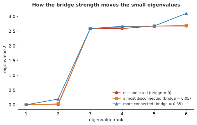
Look at the almost-disconnected curve in Figure 3.7. The first two eigenvalues sit far below the third, exactly the gap the heuristic looks for, matching what Figure 3.6 already showed: the network really does contain two natural groups.
3.11.7 Building the spectral embedding
Several low-eigenvalue coordinates give every observation a vector rather than a single number. In the normalized formulation, collect the first \(k\) symmetric eigenvectors in
\[G_k= \begin{pmatrix} |&|&&|\\ g_1&g_2&\cdots&g_k\\ |&|&&| \end{pmatrix}\]
and convert them to the random-walk coordinates
\[\boxed{ U=F_k=D^{-1/2}G_k = \begin{pmatrix} |&|&&|\\ f_1&f_2&\cdots&f_k\\ |&|&&| \end{pmatrix}. }\]
If there are \(n\) observations, then \(U\in\mathbb R^{n\times k}\). Its \(i\)th row,
\[\boxed{ U_{i\cdot} = \bigl(f_1(i),f_2(i),\ldots,f_k(i)\bigr), }\]
is observation \(i\)’s position in the spectral embedding.
Implementations vary at this last conversion. An unnormalized method uses rows of \(V_k\); normalized methods may use rows of \(F_k\), or may row-normalize the rows of \(G_k\) before label assignment. Some retain the trivial direction and others omit it. These conventions produce related but not identical embeddings, so the documentation for a particular implementation should be checked before interpreting the coordinates it returns.
For the explanation that follows, \(U=F_k\). It is the representation whose columns directly satisfy the degree-weighted smoothness problem.
3.11.8 Why connected observations stay close in spectral space
Every selected column of \(U\) was chosen because it changes slowly across strong graph connections. If observations \(A\) and \(B\) belong to the same coherent network region, we therefore tend to have
\[f_2(A)\approx f_2(B),\]
\[f_3(A)\approx f_3(B),\]
and similarly for other low-frequency eigenvectors.
So their row vectors
\[U_{A\cdot}\]
and
\[U_{B\cdot}\]
become close in the spectral embedding.
This is the goal we had from the beginning: convert graph connectivity into ordinary geometric proximity.
3.11.9 From pairwise similarities to global connectivity
Spectral clustering is not simply looking for pairs with large \(W_{ij}\).
Suppose \(A\) is strongly connected to \(B\), \(B\) to \(C\), and \(C\) to \(D\). It is possible that \(A\) and \(D\) are not directly very similar.
Nevertheless, all four observations may belong to the same coherent network region because they are connected through a chain of strong local relationships.
The low-eigenvalue eigenvectors summarize this global connectivity structure.
This is one reason spectral clustering can reveal nonlinear or manifold-like groups that ordinary centroid-based clustering may miss.
3.11.10 Why this can handle nonlinear shapes
Suppose the original observations form two concentric circles.
Ordinary \(k\)-means works directly with Euclidean coordinates and tries to describe clusters by centroids. A concentric-ring structure is therefore awkward for it.
A similarity graph changes the question.
A point on the inner circle is strongly connected to nearby points on the same circle. Those points are connected to other points on the circle, producing a coherent network component. The outer circle forms another such component.
The Laplacian eigenvectors describe these connectivity patterns rather than requiring the clusters to be linearly separated in the original feature space.
After the spectral transformation, the two ring structures may become easily separable in the new coordinates. So we can think of spectral clustering as
\[\boxed{ \text{graph-based nonlinear embedding} + \text{simple clustering in the embedding}. }\]
At this point the graph has become an ordinary geometric representation. Only the conversion from continuous points to discrete labels remains.
3.12 From the embedding to cluster labels
The graph problem is now an ordinary geometric problem. A final clustering step turns the rows of \(U\) into the labels we originally wanted.
3.12.1 Turning coordinates into labels with \(k\)-means
One gap remains. The eigenvectors provide continuous coordinates, not discrete labels.
For example, after embedding we may have
\[A\rightarrow(0.70,0.10),\]
\[B\rightarrow(0.68,0.12),\]
\[C\rightarrow(-0.30,0.71),\]
and so forth.
We still need to convert these coordinates into labels such as
\[1,1,2,2,3,3.\]
This is where a label-assignment method such as \(k\)-means is used.
In the common \(k\)-means version, \(k\)-means is not applied to the original feature space; it is applied to the spectral embedding. The workflow is
\[\boxed{ W \rightarrow D \rightarrow \text{chosen graph Laplacian} \rightarrow \text{low-eigenvalue eigenvectors} \rightarrow \text{spectral embedding} \rightarrow k\text{-means}. }\]
The substantive transformation is from the similarity graph to a useful geometry. \(k\)-means, rotation-based discretization, or another assignment rule then converts that geometry into labels.