4  Exercises: fitting and tuning spectral clustering

4.1 Setup

The dataset contains peripheral blood mononuclear cells from PBMC3k. Each row is a cell. The columns pca1 through pca10 are the inputs to clustering, while umap1 and umap2 are used only for plotting.

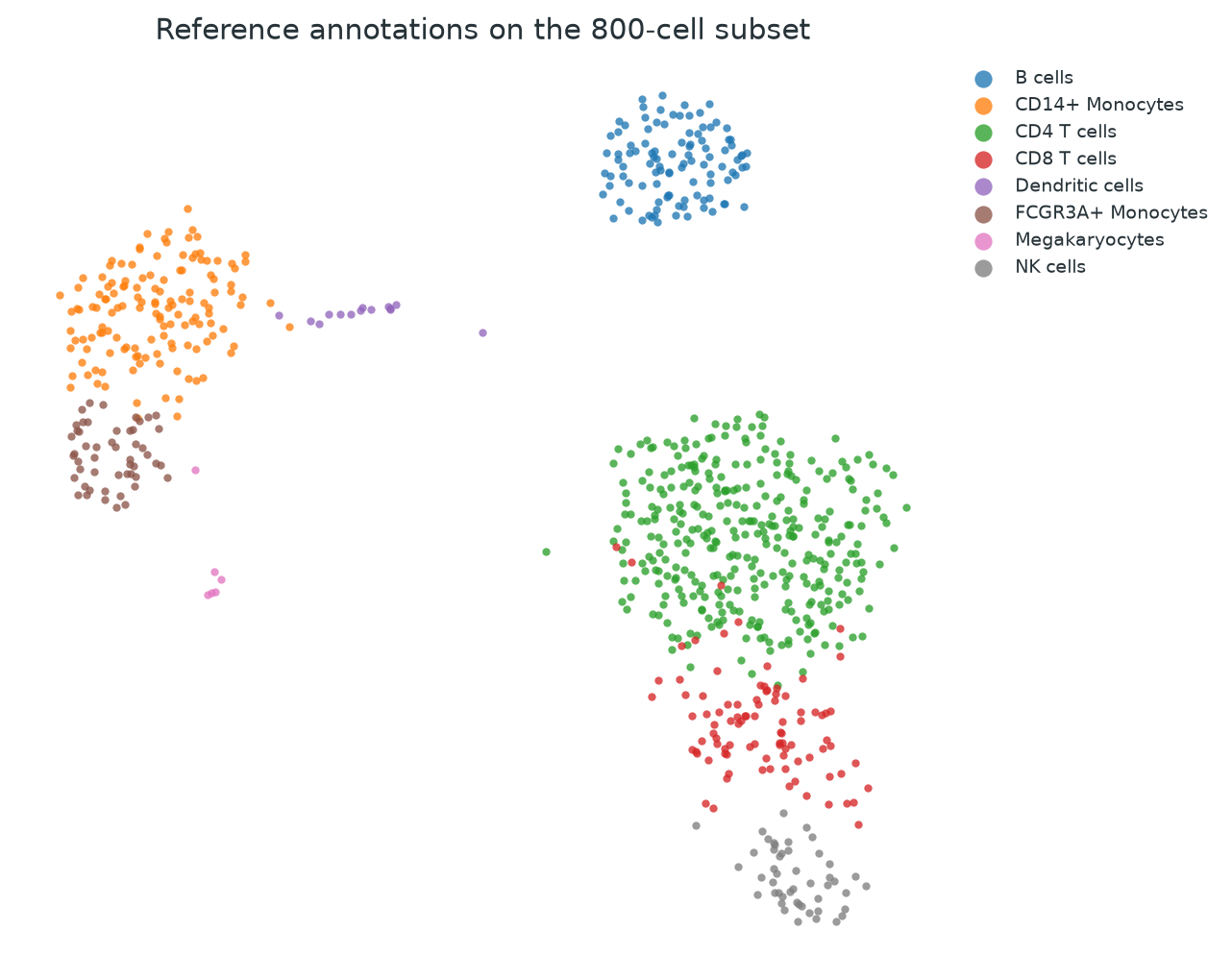
The full file contains 2,638 cells. To keep the parameter sweeps quick, both tracks use the same fixed subset: the first 800 barcode-ordered rows. The choice of rows does not use the reference annotations.

Download the two files used in the exercises:

• pbmc3k.csv — the dataset used by both R and Python
• spectral-exercise-helpers.R — the helper used to inspect spectral coordinates in the R track

Place them in a data folder beside your script or notebook so that the paths below work unchanged.

R

library(kernlab)
library(mclust)

pbmc <- read.csv("data/pbmc3k.csv")
cells <- pbmc[1:800, ]

pc_cols <- paste0("pca", 1:10)
X <- as.matrix(cells[, pc_cols])

dim(X)
table(cells$cell_type)

[1] 800  10

          B cells   CD14+ Monocytes       CD4 T cells       CD8 T cells
              105               139               344                93
  Dendritic cells FCGR3A+ Monocytes    Megakaryocytes          NK cells
               14                51                 6                48

Python

import numpy as np
import pandas as pd
import matplotlib.pyplot as plt

from sklearn.metrics import adjusted_rand_score

pbmc = pd.read_csv("data/pbmc3k.csv")
cells = pbmc.iloc[:800].copy()

pc_cols = [f"pca{i}" for i in range(1, 11)]
X = cells[pc_cols].to_numpy()

print(X.shape)
print(cells["cell_type"].value_counts())

(800, 10)
cell_type
CD4 T cells          344
CD14+ Monocytes      139
B cells              105
CD8 T cells           93
FCGR3A+ Monocytes     51
NK cells              48
Dendritic cells       14
Megakaryocytes         6
Name: count, dtype: int64

The PCA scores are used directly: standardizing the ten columns again would change the PCA geometry by giving every component equal variance. The reference annotations are available for interpretation, but they are not supplied to spectral clustering. They are not literal ground truth; they originated from a graph-based analysis and were named afterward using marker genes.

Figure 4.1: The 800-cell teaching subset on the supplied UMAP coordinates, coloured by its reference annotations.

4.2 Exercise 1. Fit spectral clustering

Fit a model with eight clusters.

• In R, use kernlab::specc() with an RBF kernel and sigma = 0.03.
• In Python, use sklearn.cluster.SpectralClustering with a nearest-neighbour affinity and n_neighbors = 10.
• Fix the random seed, count the fitted clusters, and display them on the supplied UMAP coordinates.
• Use adjusted Rand index to compare the fitted labels with cell_type.

The two packages build different affinities, so their labels and scores need not be identical.

TipHint

Cluster numbers are arbitrary. A cluster called 1 in one run can be called 6 in another without anything substantive changing. Compare membership or adjusted Rand index, not the numeric names themselves.

NoteSolution

R

set.seed(42)

fit <- specc(
  X,
  centers = 8,
  kernel = "rbfdot",
  kpar = list(sigma = 0.03),
  iterations = 100
)

labels <- as.integer(fit)

sort(table(labels), decreasing = TRUE)
round(adjustedRandIndex(cells$cell_type, labels), 4)

plot(
  cells$umap1, cells$umap2,
  col = labels, pch = 19, cex = 0.7,
  xlab = "UMAP1", ylab = "UMAP2",
  main = "kernlab::specc"
)

labels
  2   6   7   1   4   3   8   5
376 125 105  66  51  43  19  15

[1] 0.8593

Python

from sklearn.cluster import SpectralClustering

fit = SpectralClustering(
    n_clusters=8,
    affinity="nearest_neighbors",
    n_neighbors=10,
    assign_labels="kmeans",
    n_init=20,
    random_state=42,
    n_jobs=-1,
)

labels = fit.fit_predict(X)
cells["cluster"] = labels

print(pd.Series(labels).value_counts())
print(round(adjusted_rand_score(cells["cell_type"], labels), 4))

plt.scatter(
    cells["umap1"], cells["umap2"],
    c=labels, s=12, cmap="tab10"
)
plt.xlabel("UMAP1")
plt.ylabel("UMAP2")
plt.title("sklearn SpectralClustering")
plt.show()

0    210
1    140
2    134
4    106
7     90
5     61
3     45
6     14
Name: count, dtype: int64
0.6772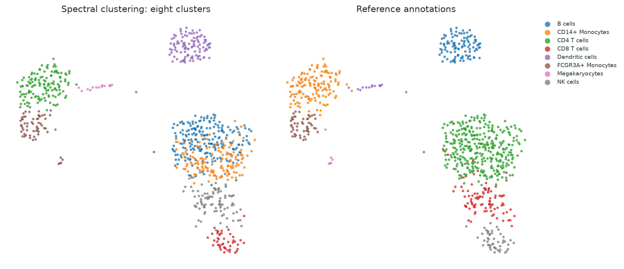

Figure 4.2: A package-based spectral clustering fit beside the reference annotations on the same UMAP display.

Both fits recover broad structure without receiving the annotations, although the two affinities divide some of the lymphocyte populations differently. The imperfect agreement is informative: several reference populations meet along continuous boundaries, and the six-cell Megakaryocyte group is very small. Asking for eight clusters does not guarantee one fitted cluster for each of eight annotation names.

4.3 Exercise 2. Tune the important parameters

A single fit does not show how strongly the result depends on its settings. First vary the affinity parameter while holding the number of clusters at eight. Then use the setting with the highest reference score and vary the number of clusters.

For R:

• try sigma values 0.001, 0.01, 0.03, 0.1, and 1;
• then hold sigma at 0.03 and try five through ten clusters.

For Python:

• try n_neighbors values 5, 10, 15, 20, and 30;
• then hold n_neighbors at 5 and try five through ten clusters.

Record the adjusted Rand index for each fit and make simple line plots. Which settings give similar agreement with the reference? Where does the score change sharply?

ImportantUsing the reference labels

The reference annotations make sensitivity easy to see in a teaching exercise. In a genuinely unsupervised analysis, using those same labels to select parameters would turn them into training information. Parameter choice would instead need stability, external outcomes, domain knowledge, or a separate labelled validation set.

NoteSolution

R

fit_specc <- function(k, sigma, seed = 42) {
  set.seed(seed)
  as.integer(specc(
    X,
    centers = k,
    kernel = "rbfdot",
    kpar = list(sigma = sigma),
    iterations = 100
  ))
}

sigma_values <- c(0.001, 0.01, 0.03, 0.1, 1)
sigma_results <- data.frame(
  sigma = sigma_values,
  ari = vapply(
    sigma_values,
    function(s) adjustedRandIndex(
      cells$cell_type,
      fit_specc(k = 8, sigma = s)
    ),
    numeric(1)
  )
)
transform(sigma_results, ari = round(ari, 4))

k_values <- 5:10
k_results <- data.frame(
  k = k_values,
  ari = vapply(
    k_values,
    function(k) adjustedRandIndex(
      cells$cell_type,
      fit_specc(k = k, sigma = 0.03)
    ),
    numeric(1)
  )
)
transform(k_results, ari = round(ari, 4))

par(mfrow = c(1, 2))
plot(sigma_results$sigma, sigma_results$ari, type = "b", log = "x",
     xlab = "RBF sigma", ylab = "ARI")
plot(k_results$k, k_results$ari, type = "b",
     xlab = "Number of clusters", ylab = "ARI")

  sigma    ari
1 0.001 0.5199
2 0.010 0.5590
3 0.030 0.8593
4 0.100 0.8057
5 1.000 0.6011

   k    ari
1  5 0.7907
2  6 0.7972
3  7 0.8031
4  8 0.8593
5  9 0.6106
6 10 0.5590

Python

def fit_spectral(k, n_neighbors, seed=42):
    model = SpectralClustering(
        n_clusters=k,
        affinity="nearest_neighbors",
        n_neighbors=n_neighbors,
        assign_labels="kmeans",
        n_init=20,
        random_state=seed,
        n_jobs=-1,
    )
    return model.fit_predict(X)

neighbor_values = [5, 10, 15, 20, 30]
neighbor_results = pd.DataFrame({
    "n_neighbors": neighbor_values,
    "ari": [
        adjusted_rand_score(
            cells["cell_type"],
            fit_spectral(k=8, n_neighbors=nn),
        )
        for nn in neighbor_values
    ],
})
print(neighbor_results.round(4))

k_values = list(range(5, 11))
k_results = pd.DataFrame({
    "k": k_values,
    "ari": [
        adjusted_rand_score(
            cells["cell_type"],
            fit_spectral(k=k, n_neighbors=5),
        )
        for k in k_values
    ],
})
print(k_results.round(4))

fig, axes = plt.subplots(1, 2, figsize=(9, 3.5))
axes[0].plot(neighbor_results["n_neighbors"], neighbor_results["ari"], marker="o")
axes[0].set(xlabel="n_neighbors", ylabel="ARI")
axes[1].plot(k_results["k"], k_results["ari"], marker="o")
axes[1].set(xlabel="Number of clusters", ylabel="ARI")
plt.tight_layout()
plt.show()

   n_neighbors     ari
0            5  0.9315
1           10  0.6772
2           15  0.6758
3           20  0.6603
4           30  0.5533

    k     ari
0   5  0.7286
1   6  0.7670
2   7  0.9297
3   8  0.9315
4   9  0.6852
5  10  0.6478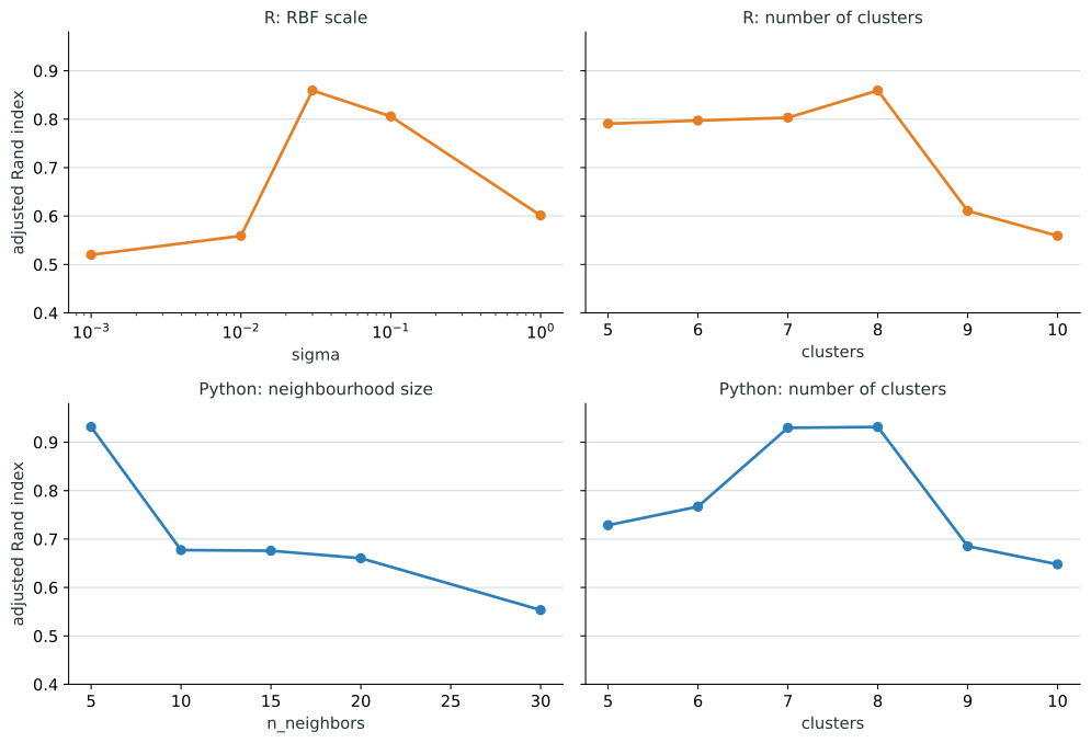

Figure 4.3: Parameter sweeps for the RBF scale and cluster count in R, and neighbourhood size and cluster count in Python.

Among the settings tested, eight clusters gives the highest agreement with the reference in both tracks. For the remaining exercises, use sigma = 0.03 in R or n_neighbors = 5 in Python, with eight clusters in either language. This is a convenient choice for the lab, not proof that eight is the uniquely correct unsupervised partition.

4.4 Exercise 3. Look at the spectral coordinates

The fitted labels are only the last output of the algorithm. Now inspect the coordinates on which that decision was based.

• Refit the selected eight-cluster model.
• Obtain its eight spectral coordinates from the same affinity.
• Plot directions 2 and 3 twice: once coloured by fitted cluster and once by reference annotation.
• Describe which populations separate cleanly and which overlap.

Scikit-learn exposes the embedding through sklearn.manifold.spectral_embedding(). The usual R specc object returns labels but not its internal coordinates, so the R track uses the provided spectral-exercise-helpers.R. Save the helper in the same data folder as the CSV. It delegates the calculation to kernlab, igraph, and RSpectra; constructing a Laplacian or solving an eigenproblem is not part of this exercise.

TipHint

An eigenvector can be multiplied by minus one without changing its meaning, and directions with nearly equal eigenvalues can rotate together. Your plot may therefore be reflected or rotated relative to the displayed solution without representing a different result.

NoteSolution

R

source("data/spectral-exercise-helpers.R")

set.seed(42)
final_fit <- specc(
  X,
  centers = 8,
  kernel = "rbfdot",
  kpar = list(sigma = 0.03),
  iterations = 100
)
final_labels <- as.integer(final_fit)

Z <- specc_embedding(
  X,
  n_components = 8,
  sigma = 0.03
)

dim(Z)
sort(table(final_labels), decreasing = TRUE)

par(mfrow = c(1, 2))
plot(
  Z[, 2], Z[, 3],
  col = final_labels, pch = 19, cex = 0.7,
  xlab = "Spectral direction 2",
  ylab = "Spectral direction 3",
  main = "Fitted clusters"
)
plot(
  Z[, 2], Z[, 3],
  col = as.integer(factor(cells$cell_type)),
  pch = 19, cex = 0.7,
  xlab = "Spectral direction 2",
  ylab = "Spectral direction 3",
  main = "Reference annotations"
)
legend(
  "topright",
  legend = levels(factor(cells$cell_type)),
  col = seq_along(levels(factor(cells$cell_type))),
  pch = 19, cex = 0.55, bty = "n"
)

[1] 800   8

final_labels
  2   6   7   1   4   3   8   5
376 125 105  66  51  43  19  15

Python

from sklearn.manifold import spectral_embedding

final_fit = SpectralClustering(
    n_clusters=8,
    affinity="nearest_neighbors",
    n_neighbors=5,
    assign_labels="kmeans",
    n_init=20,
    random_state=42,
    n_jobs=-1,
)
final_labels = final_fit.fit_predict(X)

Z = spectral_embedding(
    final_fit.affinity_matrix_,
    n_components=8,
    norm_laplacian=True,
    drop_first=False,
    random_state=42,
)

print(Z.shape)
print(pd.Series(final_labels).value_counts())

fig, axes = plt.subplots(1, 2, figsize=(10, 4))
axes[0].scatter(Z[:, 1], Z[:, 2], c=final_labels, s=12, cmap="tab10")
axes[0].set(
    xlabel="Spectral direction 2",
    ylabel="Spectral direction 3",
    title="Fitted clusters",
)

for cell_type in sorted(cells["cell_type"].unique()):
    selected = (cells["cell_type"] == cell_type).to_numpy()
    axes[1].scatter(
        Z[selected, 1], Z[selected, 2],
        s=12, label=cell_type,
    )
axes[1].set(
    xlabel="Spectral direction 2",
    ylabel="Spectral direction 3",
    title="Reference annotations",
)
axes[1].legend(frameon=False, fontsize=7, markerscale=1.5)
plt.tight_layout()
plt.show()

(800, 8)
1    352
2    132
0    106
4     86
7     60
3     47
6     12
5      5
Name: count, dtype: int64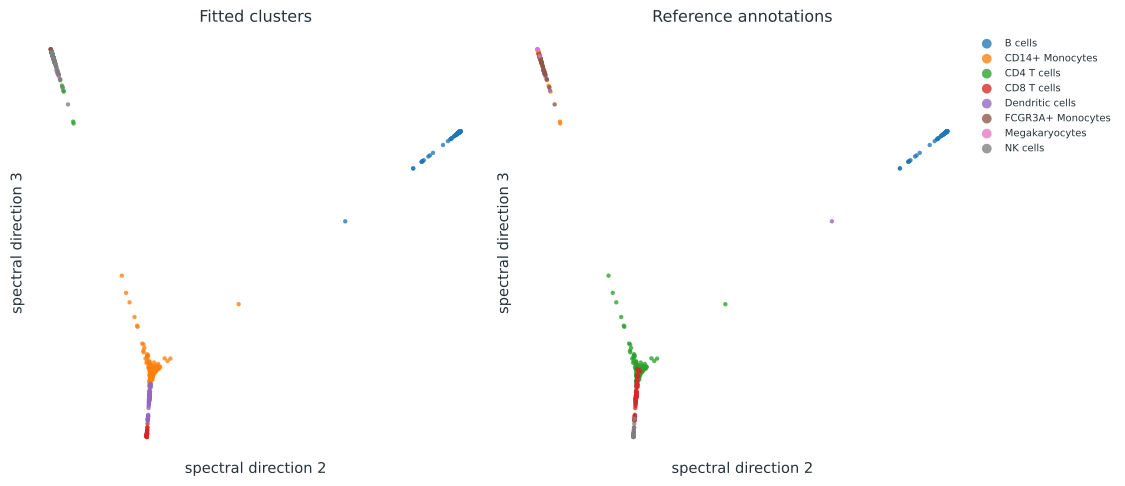

Figure 4.4: Two spectral coordinates from the selected scikit-learn model, coloured by fitted clusters and by reference annotations.

These axes are not genes, principal components, or UMAP coordinates. They are coordinates learned from connectivity in the fitted affinity graph. The first direction is associated with the graph’s trivial zero eigenvalue, which is why the plot uses directions 2 and 3. Those two axes show only one view of the eight-coordinate space used for clustering, so groups that overlap here may separate along another direction. Try plotting other pairs before deciding that two populations are inseparable.

4.5 Exercise 4. Check repeatability

The affinity and cluster count are not the only choices that can affect a result. The final label-assignment step may also depend on its random start.

Repeat the selected eight-cluster fit with seeds 1 through 5. Compare each result with the seed-42 result using adjusted Rand index. Do not use the reference annotation for this comparison.

What range of agreement do you see? Would you increase the number of starts, report the stability range, or consider a consensus result?

NoteSolution

R

repeat_labels <- lapply(1:5, function(seed) {
  fit_specc(k = 8, sigma = 0.03, seed = seed)
})

r_stability <- vapply(
  repeat_labels,
  function(candidate) adjustedRandIndex(final_labels, candidate),
  numeric(1)
)

round(r_stability, 4)
round(range(r_stability), 4)

[1] 0.8842 0.9364 0.9393 0.9713 0.8374
[1] 0.8374 0.9713

Python

repeat_labels = [
    fit_spectral(k=8, n_neighbors=5, seed=seed)
    for seed in range(1, 6)
]

py_stability = [
    adjusted_rand_score(final_labels, candidate)
    for candidate in repeat_labels
]

print(np.round(py_stability, 4))
print(min(py_stability), max(py_stability))

[1. 1. 1. 1. 1.]
1.0 1.0

For this dataset and these settings, all five Python runs agree exactly. Taking the best of 20 k-means starts within each fit helps, but it does not guarantee seed-invariant results on other data. The R fits show more variation, so repeated starts and a reported stability range should be part of that analysis.