2 Cluster evaluation in R and Python
This chapter uses three fixed expression datasets so that R and Python analyze the same observations.
- simulated_discrete_expression.csv: 300 cells, 150 genes, and three simulated populations. The labels are withheld until external comparison.
- simulated_trajectory_expression.csv: 300 cells whose expression changes continuously along pseudotime.
- simulated_null_expression.csv: 300 observations from one correlated multivariate Gaussian distribution.
The examples use cluster, ConsensusClusterPlus, fpc, and aricode in R. Python uses scikit learn for clustering and agreement, Yellowbrick for silhouette profiles, gapstatistics for Gap, consensusclustering for consensus matrices and CDF summaries, and skstab for stability.
2.1 Load and represent the discrete populations
The true population column is removed before preprocessing. We standardize genes and retain ten PCs. Ten dimensions preserve the simulated marker programs while avoiding a distance calculation dominated by 150 noisy coordinates.
library(cluster)
library(ConsensusClusterPlus)
library(fpc)
library(aricode)

set.seed(20261002)
cells <- read.csv("data/simulated_discrete_expression.csv")
truth <- cells$true_population
expression <- as.matrix(cells[grepl("^gene_", names(cells))])
pcs <- prcomp(expression, center = TRUE, scale. = TRUE)$x[, 1:10]
dim(pcs)
[1] 300 10import numpy as np
import pandas as pd
import matplotlib.pyplot as plt
from sklearn.cluster import KMeans, AgglomerativeClustering
from sklearn.decomposition import PCA
from sklearn.metrics import (
silhouette_score, silhouette_samples,
adjusted_rand_score, normalized_mutual_info_score,
adjusted_mutual_info_score
)
from sklearn.preprocessing import StandardScaler
SEED = 20261002
cells = pd.read_csv("data/simulated_discrete_expression.csv")
truth = cells["true_population"].to_numpy() # kept aside
expression = cells.filter(regex=r"^gene_").to_numpy()
pcs = PCA(n_components=10, random_state=SEED).fit_transform(
StandardScaler().fit_transform(expression)
)
print(pcs.shape)(300, 10)In an actual analysis, PC selection should use variance, technical diagnostics, and biological knowledge. Choosing the PCs by maximizing agreement with withheld labels would leak external information into model selection.
2.2 Silhouette analysis
Fit candidate values from 2 through 8 and record the mean silhouette.
candidate_k <- 2:8
fits <- lapply(candidate_k, function(k) {
  set.seed(20261002 + k)
  kmeans(pcs, centers = k, nstart = 30)$cluster
})

mean_silhouette <- vapply(
  fits,
  function(labels) mean(silhouette(labels, dist(pcs))[, "sil_width"]),
  numeric(1)
)
round(mean_silhouette, 3)
plot(candidate_k, mean_silhouette, type = "b",
     xlab = "Candidate K", ylab = "Mean silhouette")
2 3 4 5 6 7 8
0.196 0.261 0.209 0.174 0.150 0.143 0.144candidate_k = range(2, 9)
fits = {
k: KMeans(n_clusters=k, n_init=30, random_state=SEED + k).fit_predict(pcs)
for k in candidate_k
}
mean_silhouette = {
k: silhouette_score(pcs, labels) for k, labels in fits.items()
}
print({k: round(v, 3) for k, v in mean_silhouette.items()})
plt.plot(list(candidate_k), list(mean_silhouette.values()), marker="o")
plt.xlabel("Candidate K")
plt.ylabel("Mean silhouette")
plt.show(){2: 0.196, 3: 0.261, 4: 0.209, 5: 0.171, 6: 0.150, 7: 0.148, 8: 0.154}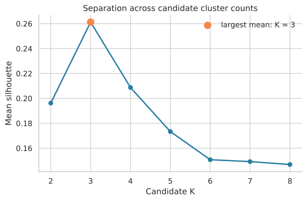
The full distribution is needed for any candidate taken forward.
par(mfrow = c(1, 3))
for (k in c(2, 3, 6)) {
  labels <- fits[[which(candidate_k == k)]]
  plot(silhouette(labels, dist(pcs)),
       main = paste("K =", k), col = 2:(k + 1), border = NA)
}

# Identify observations and assigned clusters with negative values at K = 3.
sil3 <- silhouette(fits[[2]], dist(pcs))
negative <- sil3[sil3[, "sil_width"] < 0, c("cluster", "neighbor", "sil_width")]
head(negative[order(negative[, "sil_width"]), ])
nrow(negative)
cluster neighbor sil_width
[1] 0from yellowbrick.cluster import SilhouetteVisualizer
fig, axes = plt.subplots(1, 3, figsize=(12, 4))
for ax, k in zip(axes, [2, 3, 6]):
visualizer = SilhouetteVisualizer(
KMeans(n_clusters=k, n_init=30, random_state=SEED + k),
ax=ax,
force_model=True,
colors=["#3B82F6", "#F59E0B", "#10B981", "#8B5CF6", "#EC4899", "#14B8A6"]
)
visualizer.fit(pcs)
visualizer.finalize()
ax.get_legend().remove()
ax.set_title(f"K = {k}")
ax.set(xlabel="Silhouette value", ylabel="Cluster", xlim=(-0.25, 0.9))
ax.set_xticks(np.arange(-0.2, 1.0, 0.2))
print(k, round(visualizer.silhouette_score_, 3))
plt.show()
values3 = silhouette_samples(pcs, fits[3])
negative = pd.DataFrame({
"sample_id": cells.loc[values3 < 0, "sample_id"],
"cluster": fits[3][values3 < 0],
"silhouette": values3[values3 < 0]
}).sort_values("silhouette")
print("negative silhouettes:", len(negative))
print(negative.head())2 0.196
3 0.261
6 0.150
negative silhouettes: 0
Empty DataFrame
Columns: [sample_id, cluster, silhouette]
Index: []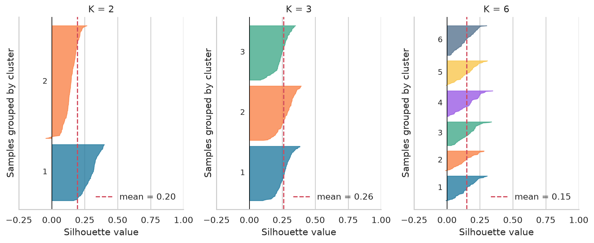
Both implementations favour \(K=3\). No observation has a negative silhouette at this resolution. The small differences at larger values of \(K\) come from implementation details in the two K means routines.
Yellowbrick 1.5 needs force_model=True with the current scikit learn estimator tags. The explicit color list avoids a removed Matplotlib colormap lookup. These compatibility settings affect the visualizer only. They do not change the silhouette values.
For millions of cells, an exact pairwise calculation can be impractical. silhouette_score accepts sample_size for a reproducible approximation. Report when an approximation or subset was used.
2.3 Gap statistic
R’s cluster::clusGap implements the classical procedure. spaceH0 = "scaledPCA" samples the reference uniformly inside a PCA aligned bounding box. maxSE(..., method = "Tibs2001SEmax") implements the original one standard error rule.
set.seed(20261002)
gap_r <- clusGap(
  pcs,
  FUNcluster = function(x, k) list(cluster = kmeans(x, k, nstart = 30)$cluster),
  K.max = 8,
  B = 100,
  spaceH0 = "scaledPCA"
)
gap_r$Tab
selected_k <- maxSE(gap_r$Tab[, "gap"], gap_r$Tab[, "SE.sim"],
                    method = "Tibs2001SEmax")
selected_k
plot(gap_r, main = "Gap statistic")
gap SE.sim
[1,] 0.412 0.011
[2,] 0.449 0.011
[3,] 0.512 0.010
[4,] 0.507 0.010
[5,] 0.510 0.010
[6,] 0.515 0.010
[7,] 0.513 0.010
[8,] 0.513 0.010
[1] 3from gapstatistics.gapstatistics import GapStatistics
np.random.seed(SEED)
gap_py = GapStatistics(pca_sampling=True, return_params=True)
selected_k, gap_params = gap_py.fit_predict(K=8, X=pcs, n_iterations=100)
gap_table = pd.DataFrame({
"K": range(1, 9),
"Gap": gap_params["gaps"],
"SE": gap_params["sim_sks"]
})
print(gap_table.round(3).to_string(index=False))
print("one-SE choice:", selected_k)
gap_py.plot() K Gap SE
1 0.591 0.009
2 0.662 0.009
3 0.749 0.009
4 0.753 0.010
5 0.761 0.010
6 0.769 0.010
7 0.768 0.010
8 0.769 0.010
one-SE choice: 3Both packages select \(K=3\) even though their Gap values differ. cluster::clusGap uses squared Euclidean within cluster dispersion. gapstatistics sums distances from observations to their assigned centroids. It also supplies its own PCA based reference sampling. The package name and its dispersion definition should accompany the reported result.
Version 0.1.5 of gapstatistics does not export GapStatistics from the package top level, so the working import uses gapstatistics.gapstatistics.
The package applies another SVD to the supplied representation and samples between one global minimum and maximum. Its Gap magnitudes can change after a numerically equivalent change in component orientation. Keep the PCA call, package version, and random seed fixed when reproducing the result.
2.4 Consensus clustering and PAC
ConsensusClusterPlus expects features in rows and items in columns. pItem = 0.8 samples 80 percent of cells per repetition. pFeature = 1 holds the representation fixed so this analysis concerns sample perturbation.
set.seed(20261002)
cc <- ConsensusClusterPlus(
  t(pcs), maxK = 8, reps = 250,
  pItem = 0.8, pFeature = 1,
  clusterAlg = "km", distance = "euclidean",
  seed = 20261002, plot = NULL, verbose = FALSE
)

pac_r <- sapply(2:8, function(k) {
  values <- cc[[k]]$consensusMatrix[upper.tri(cc[[k]]$consensusMatrix)]
  mean(values > 0.1 & values < 0.9, na.rm = TRUE)
})
round(pac_r, 3)
plot(2:8, pac_r, type = "b", xlab = "K", ylab = "PAC (0.1, 0.9)")
2 3 4 5 6 7 8
0.667 0.000 0.212 0.251 0.285 0.299 0.275from consensusclustering import ConsensusClustering
cc_py = ConsensusClustering(
KMeans(n_init=20, random_state=SEED),
min_clusters=2,
max_clusters=8,
n_resamples=100,
resample_frac=0.8,
rng=SEED
)
cc_py.fit(pcs)
auc_py = {k: cc_py.area_under_cdf(k) for k in cc_py.cluster_range_}
pac_py = {}
for k in cc_py.cluster_range_:
matrix = cc_py.consensus_k(k)
values = matrix[np.triu_indices_from(matrix, 1)]
pac_py[k] = np.mean((values > 0.1) & (values < 0.9))
print("CDF area", {k: round(v, 3) for k, v in auc_py.items()})
print("PAC", {k: round(v, 3) for k, v in pac_py.items()})
print("CDF knee:", cc_py.best_k(method="knee"))
cc_py.plot_cdf()
cc_py.plot_clustermap(3, cmap="Blues", vmin=0, vmax=1)CDF area {2: 0.504, 3: 0.700, 4: 0.747, 5: 0.800, 6: 0.849, 7: 0.866, 8: 0.880}
PAC {2: 0.446, 3: 0.000, 4: 0.128, 5: 0.200, 6: 0.156, 7: 0.166, 8: 0.167}
CDF knee: 3The numerator counts joint appearances in the same cluster. The denominator counts joint appearances. The interval (0.1, 0.9) is stated explicitly and should not be presented as a universal biological threshold.
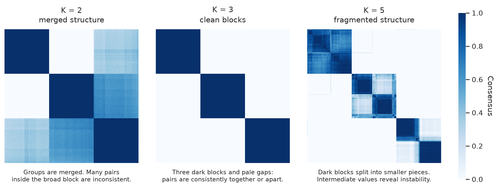
Both packages give PAC equal to zero at \(K=3\). The larger values at \(K=2\) show that merging two simulated populations creates uncertain pair assignments. The Python package also locates its CDF knee at \(K=3\). Values differ because the packages initialize and repeat K means differently. The heatmap locates ambiguous items while PAC reports their overall fraction.
2.5 Consensus on null data
Repeat the same workflow on the null matrix.
null_data <- read.csv("data/simulated_null_expression.csv")
null_expression <- as.matrix(null_data[grepl("^gene_", names(null_data))])
null_pcs <- prcomp(null_expression, center = TRUE, scale. = TRUE)$x[, 1:10]

set.seed(81)
null_cc <- ConsensusClusterPlus(
  t(null_pcs), maxK = 5, reps = 250, pItem = 0.8, pFeature = 1,
  clusterAlg = "km", distance = "euclidean",
  seed = 81, plot = NULL, verbose = FALSE
)
null_values <- null_cc[[3]]$consensusMatrix[
  upper.tri(null_cc[[3]]$consensusMatrix)
]
mean(null_values > 0.1 & null_values < 0.9, na.rm = TRUE)
[1] 0.026null_data = pd.read_csv("data/simulated_null_expression.csv")
null_expression = null_data.filter(regex=r"^gene_").to_numpy()
null_pcs = PCA(10, random_state=SEED).fit_transform(
StandardScaler().fit_transform(null_expression)
)
null_cc_py = ConsensusClustering(
KMeans(n_init=20, random_state=81),
min_clusters=3,
max_clusters=3,
n_resamples=100,
resample_frac=0.8,
rng=81
)
null_cc_py.fit(null_pcs)
null_matrix = null_cc_py.consensus_k(3)
null_values = null_matrix[np.triu_indices_from(null_matrix, 1)]
null_pac = np.mean((null_values > 0.1) & (null_values < 0.9))
print(round(null_pac, 3))0.021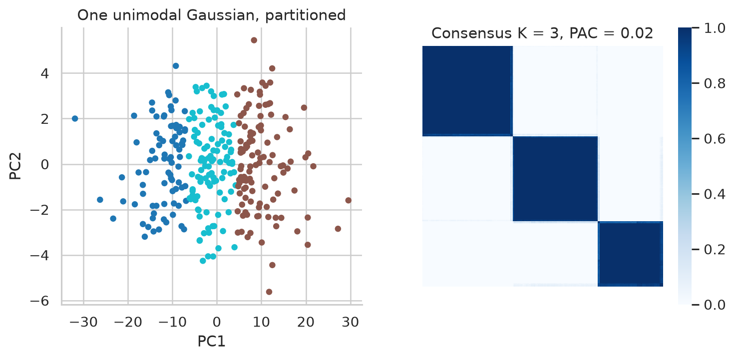
Both PAC values are low even though these data were generated from one smooth distribution. The algorithm repeatedly finds a similar forced partition. Stability therefore does not test whether discrete populations exist.
2.6 Stability
In R, clusterboot reclusters bootstrap samples and matches individual clusters by Jaccard similarity. In Python, skstab.ModelExplorer draws pairs of subsamples and compares the two complete partitions with the Fowlkes Mallows score. Its reported value is the proportion of runs whose similarity exceeds 0.9. The two packages answer related but different stability questions.
set.seed(20261002)
cb <- clusterboot(
  pcs, B = 200, bootmethod = "boot",
  clustermethod = kmeansCBI, krange = 4,
  seed = 20261002,
  count = FALSE,
  dissolution = 0.5, recover = 0.75,
  runs = 30
)
cb$bootmean
cb$bootbrd
cb$bootrecover
round(cb$bootmean, 3)
barplot(cb$bootmean, ylim = c(0, 1),
        xlab = "Original cluster", ylab = "Mean Jaccard")
abline(h = 0.75, lty = 2)
Mean Jaccard
[1] 0.686 0.826 0.904 0.664
Dissolved in 200 runs
[1] 35 3 5 89
Recovered in 200 runs
[1] 79 125 160 81from skstab import ModelExplorer
np.random.seed(SEED)
stability_py = ModelExplorer(
pcs,
KMeans,
param_name="n_clusters",
param_values=list(range(2, 9)),
f=0.8,
runs=50,
algo_kwargs={"n_init": 20, "random_state": SEED},
n_jobs=1
)
scores = stability_py.score().squeeze()
print(dict(zip(range(2, 9), np.round(scores, 3))))
plt.plot(range(2, 9), scores, marker="o")
plt.xlabel("K")
plt.ylabel("Proportion with similarity above 0.9")
plt.show(){2: 0.56, 3: 1.00, 4: 0.28, 5: 0.36, 6: 0.02, 7: 0.02, 8: 0.00}The R output shows that the four clusters at \(K=4\) do not have equal stability. The Python output compares candidate partitions and gives \(K=3\) a score of 1.00. A score of 1.00 here means that every evaluated pair of subsample fits exceeded the package threshold. It does not mean that every sample has a clusterwise Jaccard value of 1.
skstab returns singleton dimensions around this score vector. squeeze() removes those dimensions for display and does not alter the values. The current select_param() method is not used because it fails on that returned shape with the installed NumPy version.
2.7 ARI, NMI, and AMI
Only now reveal the simulated populations. Compare K means, Ward hierarchical clustering, and the withheld labels.
kmeans3 <- fits[[which(candidate_k == 3)]]
ward3 <- cutree(hclust(dist(pcs), method = "ward.D2"), k = 3)

data.frame(
  comparison = c("K-means vs truth", "Ward vs truth", "K-means vs Ward"),
  ARI = c(ARI(kmeans3, truth), ARI(ward3, truth), ARI(kmeans3, ward3)),
  NMI = c(NMI(kmeans3, truth, variant = "sum"),
          NMI(ward3, truth, variant = "sum"),
          NMI(kmeans3, ward3, variant = "sum")),
  AMI = c(AMI(kmeans3, truth), AMI(ward3, truth), AMI(kmeans3, ward3))
)
comparison ARI NMI AMI
K means vs truth 1 1 1
Ward vs truth 1 1 1
K means vs Ward 1 1 1kmeans3 = fits[3]
ward3 = AgglomerativeClustering(n_clusters=3, linkage="ward").fit_predict(pcs)
for name, left, right in [
("K means vs truth", kmeans3, truth),
("Ward vs truth", ward3, truth),
("K means vs Ward", kmeans3, ward3)
]:
print(name, {
"ARI": adjusted_rand_score(left, right),
"NMI": normalized_mutual_info_score(left, right, average_method="arithmetic"),
"AMI": adjusted_mutual_info_score(left, right, average_method="arithmetic")
})K means vs truth {'ARI': 1.0, 'NMI': 1.0, 'AMI': 1.0}
Ward vs truth {'ARI': 1.0, 'NMI': 1.0, 'AMI': 1.0}
K means vs Ward {'ARI': 1.0, 'NMI': 1.0, 'AMI': 1.0}The perfect values are a property of this deliberately clear simulation. The withheld population labels exactly match both three cluster fits. This example checks the calculation but should not be treated as a realistic expected result. The arithmetic normalizer is written explicitly in Python because NMI and AMI support several conventions. In aricode, the NMI call uses arithmetic normalization while AMI uses maximum entropy normalization. AMI and ARI are chance corrected. NMI is not.
2.7.1 Splits and merges
A <- as.integer(factor(c("A", "A", "A", "B", "B", "B", "C", "C")))
B_split <- c(1, 1, 1, 2, 3, 4, 5, 5)
C_merge <- c(1, 1, 1, 2, 2, 2, 2, 2)

table(A, B_split)
c(ARI = ARI(A, B_split), AMI = AMI(A, B_split))
table(A, C_merge)
c(ARI = ARI(A, C_merge), AMI = AMI(A, C_merge))
Split table
B_split
A 1 2 3 4 5
1 3 0 0 0 0
2 0 1 1 1 0
3 0 0 0 0 2
ARI AMI
0.667 0.502
Merge table
C_merge
A 1 2
1 3 0
2 0 3
3 0 2
ARI AMI
0.556 0.531A = np.array(list("AAABBBCC"))
B_split = np.array([1, 1, 1, 2, 3, 4, 5, 5])
C_merge = np.array([1, 1, 1, 2, 2, 2, 2, 2])
print(pd.crosstab(A, B_split))
print({
"ARI": adjusted_rand_score(A, B_split),
"NMI": normalized_mutual_info_score(A, B_split),
"AMI": adjusted_mutual_info_score(A, B_split)
})
print(pd.crosstab(A, C_merge))
print({
"ARI": adjusted_rand_score(A, C_merge),
"NMI": normalized_mutual_info_score(A, C_merge),
"AMI": adjusted_mutual_info_score(A, C_merge)
})Split table
col_0 1 2 3 4 5
row_0
A 3 0 0 0 0
B 0 1 1 1 0
C 0 0 0 0 2
{'ARI': 0.667, 'NMI': 0.840, 'AMI': 0.669}
Merge table
col_0 1 2
row_0
A 3 0
B 0 3
C 0 2
{'ARI': 0.556, 'NMI': 0.759, 'AMI': 0.694}The tables show which original group was split or merged. The scores summarize the whole partition and cannot identify that source by themselves.
2.8 Representation sensitivity
Repeat the silhouette sweep in the standardized 150 gene matrix, the first two PCs, and the first ten PCs.
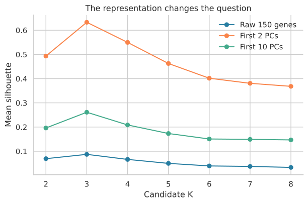
The same validation function in Figure 2.5 evaluates three different geometries. PCA is not guaranteed to be best. The point is to report where distances were calculated and to keep that representation connected to the clustering procedure.
2.9 Parameters other than K
The same workflow can evaluate a resolution parameter. For Leiden, fit a short range of resolution values and record the number of returned clusters, mean silhouette in the chosen representation, and a stability summary. This does not turn resolution into \(K\). Several settings can return the same count with different memberships.
DBSCAN should be evaluated across eps and MinPts, including the proportion labeled as noise. HDBSCAN determines groups through its density hierarchy. For these methods, forcing a \(K\) selection framework would ignore how the algorithm works.
The mathematical chapter now derives every quantity used here.