5 Random forest
Before starting let’s have a look at our aggregated variance formula again:
\[p\sigma^2+\frac{1-p}{m}\sigma^2\] We said that if we have a large \(m\), we will end up having \(p\sigma^2\) as our aggregated variance. In this formula, \(p\) is the pairwise correlation between the trees. We know that \(0\le p \le 1\) so obviously as we decrease \(p\) toward \(0\) we at the same time decrease \(p\sigma^2\). So how do we decrease our variance in bagging even further? We decrease the correlation between different trees. That is exactly what Random forest does. Random forest adds another level of randomness to the process of building the tree so that trees have lower correlations. This is how random forest works:
Let’s say we have a dataset with \(N\) number of samples and \(p\) number of features. To build a random forest model we do:
Take a random sample of size \(N\) with replacement from the data (similar to bagging).
Now for finding a split, we take a random sample of \(k\) variables from \(p\) without replacement and use only this subset of variables to find the best split. This is the random part of random forest.
To further split this tree, repeat step 2 until the tree is large enough.
Repeat steps 1 to 3 many times to produce more trees. This is the forest part of random forest
Similar to bagging, we predict each sample to a final group by a majority vote over the set of trees. For example, if we have 500 trees and 400 of them say sample \(x\) is AD, then we use this as the predicted group for the sample \(x\). For regression, we simply take the mean of all the predicted values of all the 500 trees.
So the only additional component here is focusing on a random subset of our features or variables when doing a split. It should be apparent now that random forests can reduce the variance as the direct result of bagging and random splits. In addition, they can also deal with very large datasets especially when the number of variables is large and even greater than the number of samples. Finally, random forests can highlight out-competed variables. The effects of these variables are often cancelled out by other more dominant variables. However, with random forests (with large trees), they will have a chance of to a node in at least some of the trees.
We are now ready to start coding random forests. We will be used randomForest function from randomForest package.
library(ipred)
library(rpart)
par(mfrow=c(1,2))
set.seed(20)
testing_index<-sample(1:length(data$p_tau),100,replace = F)

limited_data4_training<-data[-testing_index,]
limited_data4_testing<-data[testing_index,]

limited_data4_training$group<-as.factor(limited_data4_training$group)
limited_data4_training$gender<-as.factor(limited_data4_training$gender)

limited_data4_testing$group<-as.factor(limited_data4_testing$group)
limited_data4_testing$gender<-as.factor(limited_data4_testing$gender)

set.seed(10)
bagged_model <- bagging(group ~ ., data = limited_data4_training,nbagg=100)


set.seed(10)
tree_model <- rpart(group ~ ., data = limited_data4_training,
   method="class")
set.seed(10)
tree_model<- prune(tree_model, cp=   tree_model$cptable[which.min(tree_model$cptable[,"xerror"]),"CP"])

set.seed(10)
rf_model<-randomForest::randomForest(group ~ ., data = limited_data4_training,ntree=100,importance=T)


acc_bagging<-mean(limited_data4_testing$group == predict(bagged_model,limited_data4_testing,type = "class"))

acc_tree<-mean(limited_data4_testing$group == predict(tree_model,limited_data4_testing,type = "class"))

acc_rf<-mean(limited_data4_testing$group == predict(rf_model,limited_data4_testing[,-7],type = "class"))


confMatrix_bagging<-caret::confusionMatrix(predict(bagged_model,limited_data4_testing[,-7],type = "class"),limited_data4_testing$group )
confMatrix_tree<-caret::confusionMatrix(predict(tree_model,limited_data4_testing[,-7],type = "class"),limited_data4_testing$group )
confMatrix_rf<-caret::confusionMatrix(predict(rf_model,limited_data4_testing[,-7],type = "class"),limited_data4_testing$group )


plot_data<-rbind(data.frame(reshape::melt(confMatrix_bagging$table),Method="Bagging"),
      data.frame(reshape::melt(confMatrix_tree$table),Method="Normal"),data.frame(reshape::melt(confMatrix_rf$table),Method="RandomForest"))
names(plot_data)[1:2]<-c("x","y")
plot_data$Color=NA
plot_data$Color[plot_data$x==plot_data$y]<-"red"
library(ggplot2)

ggplot(plot_data, aes(Method,fill=Method)) +
    geom_bar(aes(y = value),
             stat = "identity"#, position = "dodge"
             ) +
    geom_text(aes(y = -5, label = value,color=Method)) +
    facet_grid(x ~ y, switch = "y") +
    labs(title = "",
         y = "Predicted class",
         x = "True class") +
    theme_bw() +
   geom_rect(data=plot_data, aes(fill=Color), xmin=-Inf, xmax=Inf, ymin=-Inf, ymax=Inf, alpha=0.095)+
  scale_fill_manual(values=c("blue", "red","green","red"), breaks=NULL)+
    scale_color_manual(values=c("blue", "red","green"), breaks=NULL)+
    theme(strip.background = element_blank(),panel.border = element_rect(color = , fill = NA, size = 1),
          axis.text.y = element_blank(),
          axis.text.x = element_text(size = 9),
          axis.ticks = element_blank(),
          strip.text.y = element_text(angle = 0),
          strip.text = element_text(size = 9))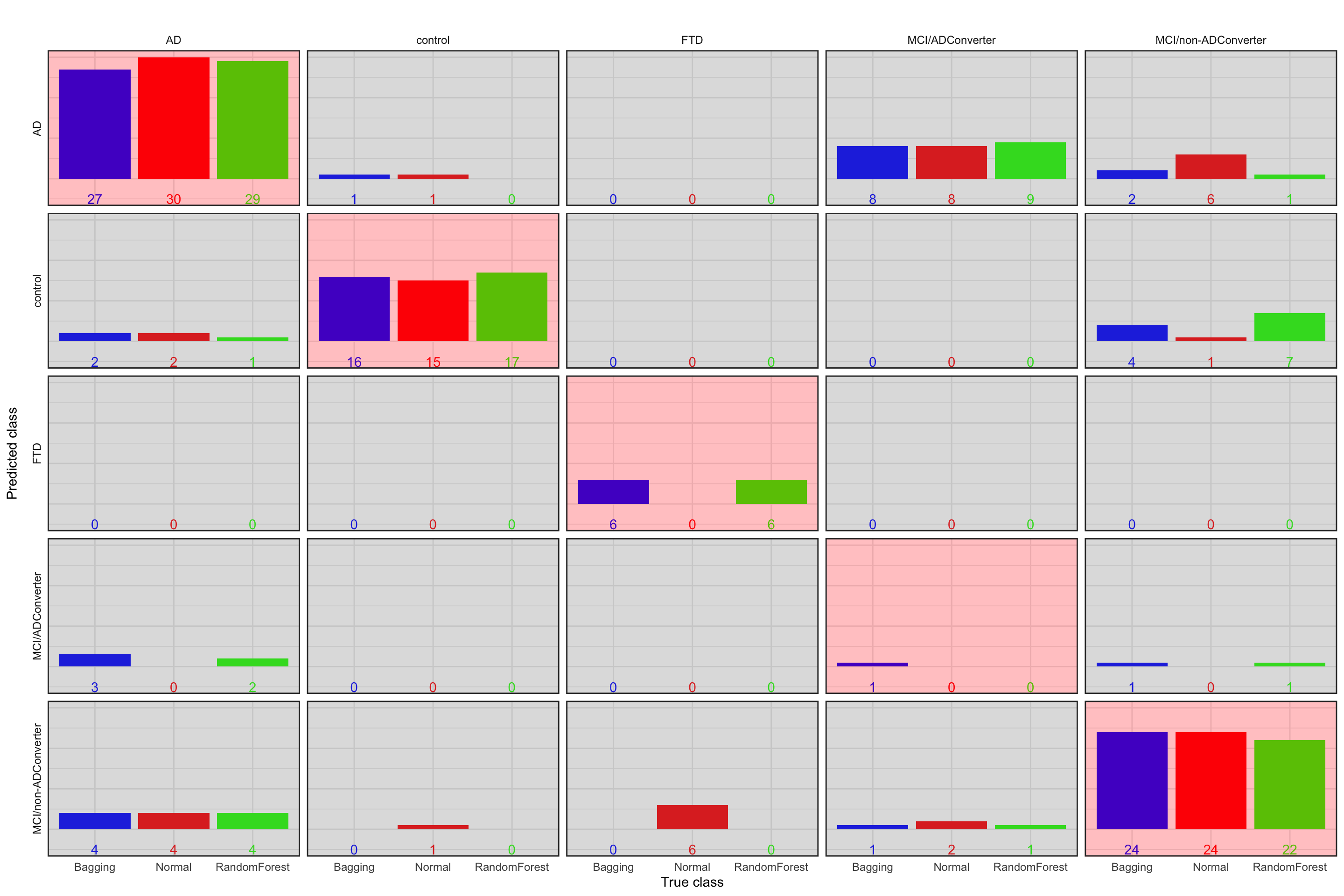
Figure 5.1: Prediction accuracy of normal tree vs. bagging vs. random forest. Blue bar: Bagging, red bar: Normal, green bar: random forest. The plots with red background are correct classification
In this case, random forest performs slightly better (accuracy=0.75) than others. Please note that this specific dataset is very small so all the methods are expected to work similarly. Nevertheless, the random forest algorithm is performing fairly good.
Random forests just like many other statistical models have some parameters and need to be tuned. In the case of random forest, these parameters are:
- The number of samples in each leaf node (
nodesizeinrandomForestpackage). - Number of trees (
ntreeinrandomForestpackage). - Number of variables to consider at each split (
mtryinrandomForestpackage).
Please note that we don’t do pruning in random forests and nodesize should be used with care to not building too shallow trees. In the next section, we try to tune mtry and ntree.
5.1 Tuning parameters for random forests
As we discussed before, cross-validation can be used to tune parameters for statistical models. We can also use them for tuning mtry and ntree. An easier way to do so is to use out of bag error. We show both of our approaches here. Although there are packages like caret that automate this process, we use a manual approach so you can see how it is done.
library(ipred)
library(rpart)
set.seed(20)
testing_index<-sample(1:length(data$p_tau),100,replace = F)

limited_data4_training<-data[-testing_index,]
limited_data4_testing<-data[testing_index,]

limited_data4_training$group<-as.factor(limited_data4_training$group)
limited_data4_training$gender<-as.factor(limited_data4_training$gender)

limited_data4_testing$group<-as.factor(limited_data4_testing$group)
limited_data4_testing$gender<-as.factor(limited_data4_testing$gender)


# Create grid of search parameters
hp_grid <- expand.grid(
  mtry       = c(2:5),
  ntree = seq(100, 500, by = 100),
  OOB  = 0,
  CV = 0
)

# loop over each hpyper parameter
for(i in 1:nrow(hp_grid)) {

  # train model
  set.seed(i)
rf_model<-randomForest::randomForest(group ~ ., data = limited_data4_training,ntree=hp_grid$ntree[i],mtry=hp_grid$mtry[i],importance=T)

set.seed(i)
folds <- sample(rep(1:5, length.out = nrow(limited_data4_training)), size = nrow(limited_data4_training), replace = F)

CV_rf <- sapply(1:5, function(x){
  tmp<-limited_data4_training[folds != x,]
  set.seed(i*x)
  model <- randomForest::randomForest(group ~ ., data =limited_data4_training[folds != x,] ,ntree=hp_grid$ntree[i],mtry=hp_grid$mtry[i],importance=T)

  return( 100-(caret::confusionMatrix(predict(model,limited_data4_training[folds== x,],type="response"), limited_data4_training[folds== x,"group"] )$overall[1]*100))
  })

hp_grid$OOB[i] <- round(rf_model$err.rate[rf_model$ntree,"OOB"] * 100, digits = 2)
hp_grid$CV[i]<-median(CV_rf)
}

hp_grid$ntree<-factor(hp_grid$ntree)
oob_plot<-ggplot(data = hp_grid, aes(x=mtry, y=OOB)) +geom_point(aes(colour=ntree))+ geom_line(aes(colour=ntree))+theme_classic()+ylim(min(c(hp_grid$OOB,hp_grid$CV)),max(c(hp_grid$OOB,hp_grid$CV)))
cv_plot<-ggplot(data = hp_grid, aes(x=mtry, y=CV)) +geom_point(aes(colour=ntree))+ geom_line(aes(colour=ntree))+theme_classic()+ylim(min(c(hp_grid$OOB,hp_grid$CV)),max(c(hp_grid$OOB,hp_grid$CV)))
cowplot::plot_grid(oob_plot,cv_plot,labels = c("A","B"))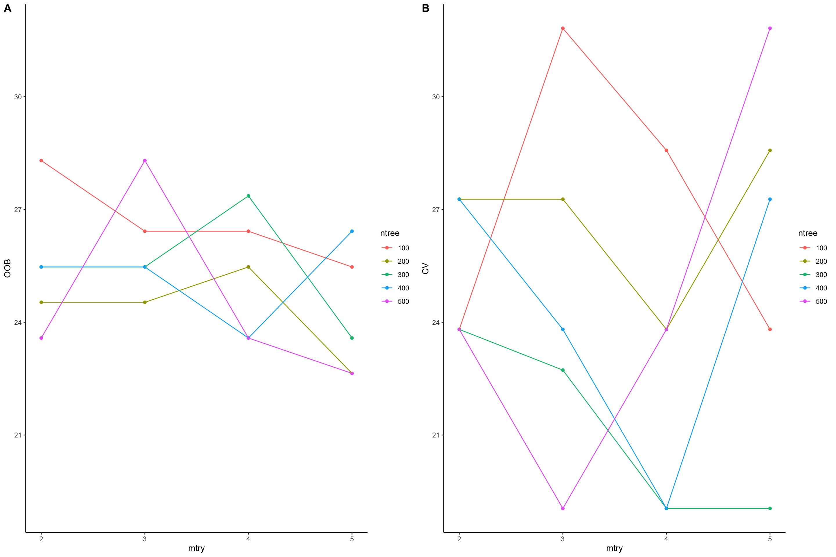
Figure 5.2: Paramemter tuning for mtry and ntree. Out of bag errors (A) are compared with cross validation (B)
In the plot above, we have plotted out of bag error (OOB) and cross validation error (CV) vs mtry. In out of bag error (plot A), we see that mtry: 5 and ntree: 200 have minimize the error rate: 22.64. In plot B, we present the median error rate of 5-fold cross validation. We see that mtry: 4 and ntree: 300 have minimize the error rate: 19.0476190476191. So cross validation has minimize the error rate so we can probably use the parameters suggested by cross validation. In practice however, having too few samples, out of bag is probably more preferable that cross validation.
5.2 Variable importance
Random forests are not only used for doing prediction but they provide a very powerful framework for variable selection. Variable selection or feature importance refers to the process of finding what variables have the most influence on the outcome of the model. So a researcher might as if I can diagnose a type of cancer with very good accuracy what are the genes that are more important for doing that prediction? This type of question can be answered by variable selection. In random forests, there are two major ways to find the importance of a variable. One is based on the mean increase in prediction error via permutation and the second one is the decrease in node impurity. Both of these can be calculated either by setting importance=TRUE in the main randomForest function or by directly using importance function. Let’s first talk about how they are calculated.
5.2.1 Feature importance by permutation
To calculate the feature importance by permutation, one can use both cross-validation and out of bag errors. Here we focus on out of bag errors:
Let’s say that we trained a model \(f\) on our data \(X\) on response \(y\). As we said before, we can calculate out of bag errors (OOB) for this model. Let’s call this \(OOB^{\ orig}\) and calculate it using an error measure \(E\) so: \(OOB^{\ orig}=E(y-f(X))\). Now, for each of the features \(i=1,...,p\), we do a random permutation (shuffling) and put it back in the original matrix. Let’s call this matrix \(X^{perm}_i\). This means all other features are original ones except feature \(i\) that has been randomly shuffled. We can now calculate the out of bag error for this new data \(OOB^{\ perm}_i=E(y-f(X^{perm}_i))\). In the last step, we calculate the difference between the original out of bag error vs. the permuted out of bag error: \(dif_i=OOB^{\ perm}_i-OOB^{\ orig}\). We do this for all the features, one at a time giving us the list of permuted \(OOB^{\ perm}_i ,\ i=1,...,p\). In the last step, we normalize this by the standard deviation of \(OOB^{\ perm}\) and sorting by descending order.
To put it simply, we ask the question that if we shuffle this specific feature, how much our model become poorer than the original model. If a feature makes our model becomes worse a lot, it has more influence on the model thus it is more important. By sorting these influences we can rank our variables according to their importance. One great this about this way of finding feature importance is that we can also calculate \(OOB\) not only for all the samples but for each class of the samples (e.g., AD or control) giving us feature importance for predicting a specific group of samples.
5.2.2 Feature importance by impurity
Feature importance by impurity does not take into account the out of bag error or cross-validation but rather asks the question of how much throughout the tree a specific feature has been decreasing the impurity.
If you remember, we calculate a node Gini impurity by \(\text{Gini impurity}=1-\sum_{i}^{C}{p(i)^2}\) and entropy by \(\text{Entropy}=1-\sum_{i}^{C}{p(i)log{_2}{p(i)}}\), for classification and for regression by \(MSE=\frac{1}{n}\sum_{i=1}^{n}{(y_i-\bar{y_i})^2}\) or by residual sum of squares. At this stage, no matter what we use, we want to call this \(IMP_j\) where \(j\) can be any node in the tree. And if you remember, we calculate the weighted removed impurity of a parent node as:
\[RI_j=W_j\times IMP_j-W_{left_j}\times IMP_{left_j}-W_{right_j}\times IMP_{right_j}\]
where \(W_{j}\) is the weight of the parent node (e.g \(\frac{N(j)}{N}\); proportion data coming into node \(j\)). \(W_{left_j}\) is the weight of the left child node \(j\) (see aggregating Gini above). Please note that in some implementations \(W_j\) has been removed.
Now what we have is the decrease in impurity for each node but we are interested in features not nodes! We define another measure as average feature impurity decrease:
\[FIMP_i=\frac{\sum_{j \in N_i}{RI_j}}{\sum_{k \in t}{RI_k}}\] Where \(N_i\) is all the nodes where feature \(i\) has been used to split the node and \(t\) is the set of all nodes in the tree. We can then normalize this \(FIMP_i\) by the sum of all \(FIMP_i\) giving us:
\[FIMP^{\ norm}_i=\frac{FIMP_i}{\sum_i^p{FIMP_i}}\] Finally, as we build multiple trees in random forest, we have to calculate the average feature importance across all the trees:
\[FI_i=\frac{\sum_{j\in trees}{{FIMP^{\ norm}_{i,j}}}}{|T|}\] where \(FI_i\) is the feature importance of variable \(i\), \(FIMP^{\ norm}_{i,j}\) is the normalized \(FIMP\) for feature \(i\) in tree \(j\) and \(|T|\) is the total number of trees. What the whole thing is telling us is that for each feature in each tree, we calculate the average decrease in impurity, sum it over the trees and normalize it by the number of trees.
Please note that there are many different implementation feature importance but in principle, most of them are very similar to what we have discussed so far.
We can now have a look at our feature importance in random forest:
library(ipred)
library(rpart)
set.seed(20)
testing_index<-sample(1:length(data$p_tau),100,replace = F)

limited_data4_training<-data[-testing_index,]
limited_data4_testing<-data[testing_index,]

limited_data4_training$group<-as.factor(limited_data4_training$group)
limited_data4_training$gender<-as.factor(limited_data4_training$gender)

rf_model<-randomForest::randomForest(group ~ ., data = limited_data4_training,ntree=100,importance=T)
randomForest::varImpPlot(rf_model)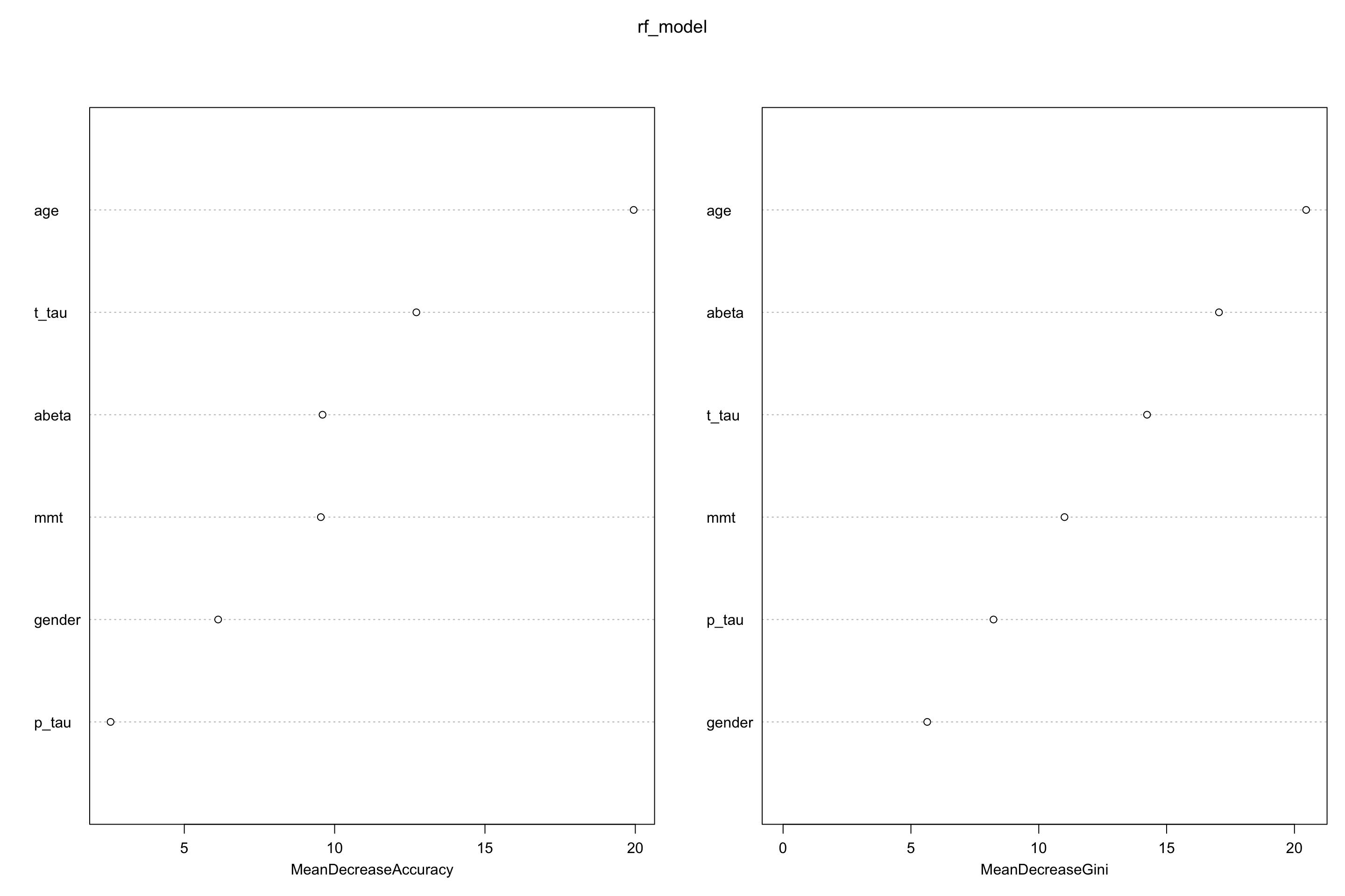
Figure 5.3: Feature importance for random forests
Both mean decrease in accuracy (left plot) and impurity base (right plot) are plotted here. We see that our top tree features are age, t-tau and \(A\beta\). Mean decrease in accuracy tells us that t-tau is more important that \(A\beta\) but Gini tells the opposite. We can use any of these to select our variables.
5.3 How to use random forest in R
There are many packages for random forest. We have been using randomForest package in R that does a decent job and is fast enough for most of the applications. There are other implementations that you can check out such as ranger that is even faster. We here go through randomForest package briefly.
5.3.1 Data
Our data has to be in a data.frame where features are in the columns and samples in the rows. The categorical variables should preferably be factor and you should have a column for your response variable. You can then use formula capability of R to easily run randomForest: randomForest::randomForest(group ~ ., data = limited_data4_training). This essentially says that our data is sitting in a data frame which has a called named group. The dot in from of tilde (~) tells the formula the use all other columns (except group) for modelling the data. This is how our data look like:
##    gender age mmt abeta t_tau p_tau group
## 1       M  75  12   370   240    44    AD
## 4       F  82  26   230   530    84    AD
## 7       M  70  25   270   230    34    AD
## 9       F  68  27   160   810   100    AD
## 11      M  77  23   430   780   119    AD
## 12      F  80  26   350  1150   159    AD
You can set various parameters in randomForest but probably the most relevant ones are mtry, ntree and importance. We have already covered all of these and in one command you can run randomForest::randomForest(group ~ ., data = limited_data4_training,mtry=5,ntree=100).
set.seed(20)
testing_index<-sample(1:length(data$p_tau),100,replace = F)

limited_data4_training<-data[-testing_index,]
limited_data4_testing<-data[testing_index,]

limited_data4_training$group<-as.factor(limited_data4_training$group)
limited_data4_training$gender<-as.factor(limited_data4_training$gender)

limited_data4_testing$group<-as.factor(limited_data4_testing$group)
limited_data4_testing$gender<-as.factor(limited_data4_testing$gender)

rf_model<-randomForest::randomForest(group ~ ., data = limited_data4_training,ntree=100,importance=T)

print(rf_model)
##
## Call:
## randomForest(formula = group ~ ., data = limited_data4_training, ntree = 100, importance = T)
## Type of random forest: classification
## Number of trees: 100
## No. of variables tried at each split: 2
##
## OOB estimate of error rate: 28.3%
## Confusion matrix:
## AD control FTD MCI/ADConverter MCI/non-ADConverter
## AD 36 2 0 0 2
## control 4 23 0 0 1
## FTD 1 0 0 0 4
## MCI/ADConverter 9 1 0 0 1
## MCI/non-ADConverter 3 2 0 0 17
## class.error
## AD 0.1000000
## control 0.1785714
## FTD 1.0000000
## MCI/ADConverter 1.0000000
## MCI/non-ADConverter 0.2272727For doing prediction, we will use predict function. This function has three main arguments:object, newdata and type. object is the model we have trained. newdata is the data.frame of our new data and type is one of response, prob. or votes, indicating the type of output: predicted values, matrix of class probabilities, or matrix of vote counts.
##                 166                 191                 107                 120
##             control             control             control MCI/non-ADConverter
##                 130                  98
## MCI/non-ADConverter                  AD
## Levels: AD control FTD MCI/ADConverter MCI/non-ADConverter
We can use confusionMatrix function from caret package to calculate some accuracy measures. This function gets the predicted and true values caret::confusionMatrix((predicted_class,true_class)
## Confusion Matrix and Statistics
##
##                      Reference
## Prediction            AD control FTD MCI/ADConverter MCI/non-ADConverter
##   AD                  30       1   0               9                   3
##   control              0      16   0               0                   6
##   FTD                  0       0   3               0                   0
##   MCI/ADConverter      2       0   0               0                   0
##   MCI/non-ADConverter  4       0   3               1                  22
##
## Overall Statistics
##
##                Accuracy : 0.71
##                  95% CI : (0.6107, 0.7964)
##     No Information Rate : 0.36
##     P-Value [Acc > NIR] : 1.203e-12
##
##                   Kappa : 0.5921
##
##  Mcnemar's Test P-Value : NA
##
## Statistics by Class:
##
##                      Class: AD Class: control Class: FTD Class: MCI/ADConverter
## Sensitivity             0.8333         0.9412     0.5000                 0.0000
## Specificity             0.7969         0.9277     1.0000                 0.9778
## Pos Pred Value          0.6977         0.7273     1.0000                 0.0000
## Neg Pred Value          0.8947         0.9872     0.9691                 0.8980
## Prevalence              0.3600         0.1700     0.0600                 0.1000
## Detection Rate          0.3000         0.1600     0.0300                 0.0000
## Detection Prevalence    0.4300         0.2200     0.0300                 0.0200
## Balanced Accuracy       0.8151         0.9344     0.7500                 0.4889
##                      Class: MCI/non-ADConverter
## Sensitivity                              0.7097
## Specificity                              0.8841
## Pos Pred Value                           0.7333
## Neg Pred Value                           0.8714
## Prevalence                               0.3100
## Detection Rate                           0.2200
## Detection Prevalence                     0.3000
## Balanced Accuracy                        0.7969
To tune mtry we can use tuneRF from randomForest. This function gets multiple arguments including x: data without the class (group) column, y: group columns, mtryStart: starting value of mtry, ntreeTry: number of trees to build. It will use out of bag error to calculate tuned value for mtry. However, for tuning other parameters we might need to write our own function or use other packages such as caret.
par(mfrow=c(1,1))
set.seed(5)
randomForest::tuneRF(limited_data4_training,limited_data4_training$group,mtryStart = 1)
## mtry = 1 OOB error = 8.49%
## Searching left ...
## Searching right ...
## mtry = 2 OOB error = 2.83%
## 0.6666667 0.05
## mtry = 4 OOB error = 0.94%
## 0.6666667 0.05
## mtry = 7 OOB error = 0%
## 1 0.05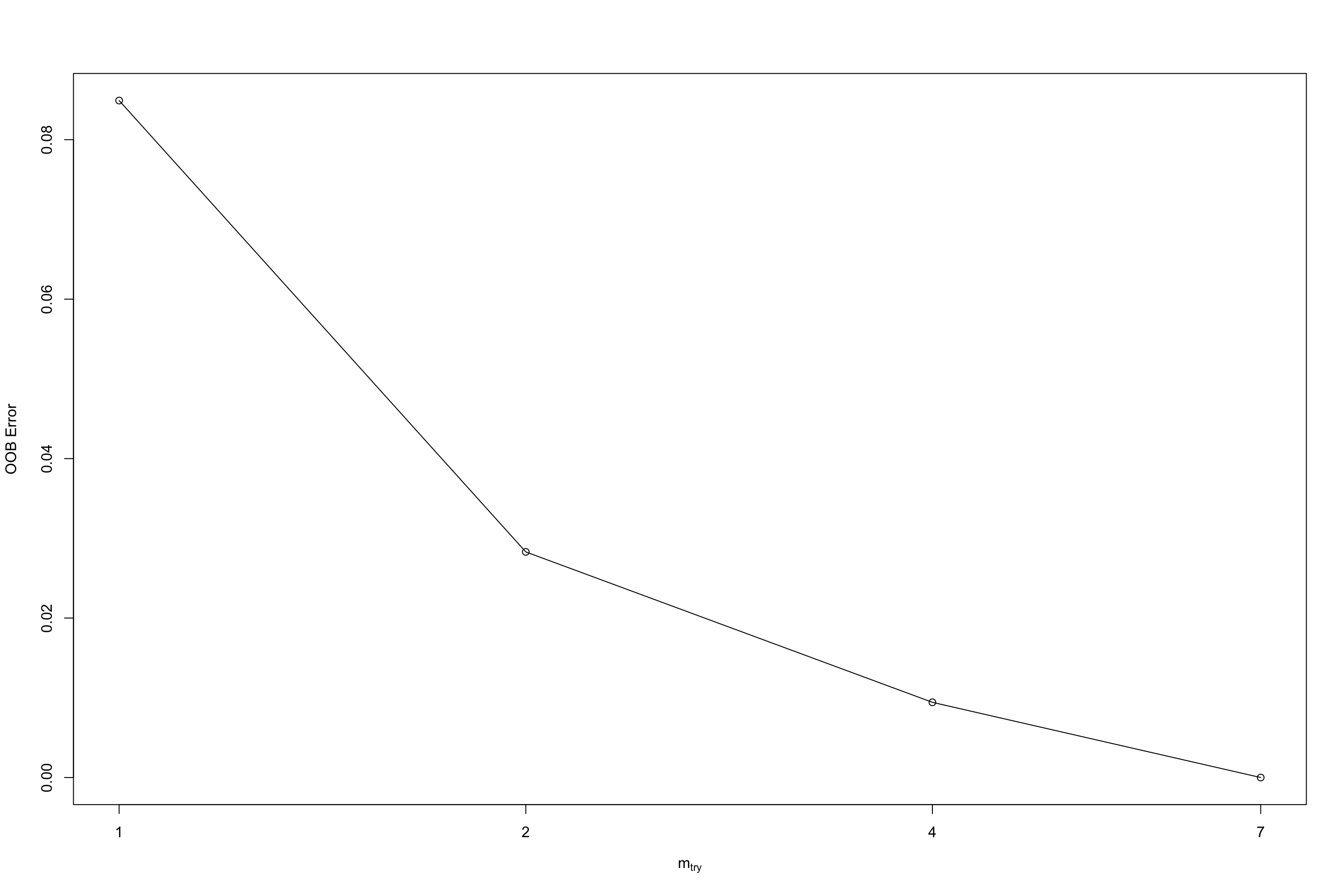
Figure 5.4: Tuning output of tuneRF
##       mtry    OOBError
## 1.OOB    1 0.084905660
## 2.OOB    2 0.028301887
## 4.OOB    4 0.009433962
## 7.OOB    7 0.000000000
Finally, to see the variable importance, we can use importance and varImpPlot function to extract and plot the variable importance. There are multiple parameters but the most important ones are x: random forest model, type: either 1 or 2, specifying the type of importance measure (1=mean decrease in accuracy, 2=mean decrease in node impurity), class: for the classification problem, which class-specific measure to return.
##               AD   control        FTD MCI/ADConverter MCI/non-ADConverter
## gender 0.2606584  4.118921  5.8516194      -0.2829469            2.632055
## age    5.4417838 21.579161  1.5053292       3.7648161            7.118233
## mmt    5.7195419  7.764001 -0.2705999       1.0383546            3.816802
## abeta  5.6091130  3.494602 -1.3176872      -0.3068971            9.856776
## t_tau  7.2440944  2.719246 -2.2393747      -0.2076253           13.324209
## p_tau  0.4144791  1.788861  0.7930516       0.1244211            3.053540
##        MeanDecreaseAccuracy MeanDecreaseGini
## gender             6.125677         5.636911
## age               19.944318        20.457114
## mmt                9.541772        11.006211
## abeta              9.598139        17.047667
## t_tau             12.718459        14.234984
## p_tau              2.548707         8.229038
Figure 5.5: Variable importance plot