4 Bagging
4.1 Bias-variance
Let’s first think about the overfitting problem we went through before.
par(mfrow=c(1,2))
set.seed(20)
testing_index<-sample(1:length(limited_data$p_tau),50,replace = F)

limited_data4_training<-limited_data[-testing_index,]
limited_data4_testing<-limited_data[testing_index,]


lw1 <- loess(t_tau ~ p_tau,data=limited_data4_training,span = 0.1)
cor1<-cor(limited_data4_testing$t_tau,predict(lw1,limited_data4_testing$p_tau),use = "p")^2

j <- order(limited_data4_training$p_tau)
plot(limited_data4_training$p_tau,limited_data4_training$t_tau,xlab = "p-tau",ylab = "t-tau",main = paste("R2:", round(cor1,digits = 2)))

lines(limited_data4_training$p_tau[j],lw1$fitted[j],col="red",lwd=3)


lw1 <- loess(t_tau ~ p_tau,data=limited_data4_training,span = 0.6)
cor2<-cor(limited_data4_testing$t_tau,predict(lw1,limited_data4_testing$p_tau),use = "p")^2
plot(limited_data4_training$p_tau,limited_data4_training$t_tau,xlab = "p-tau",ylab = "t-tau",main = paste("R2:", round(cor2,digits = 2)))
j <- order(limited_data4_training$p_tau)
lines(limited_data4_training$p_tau[j],lw1$fitted[j],col="red",lwd=3)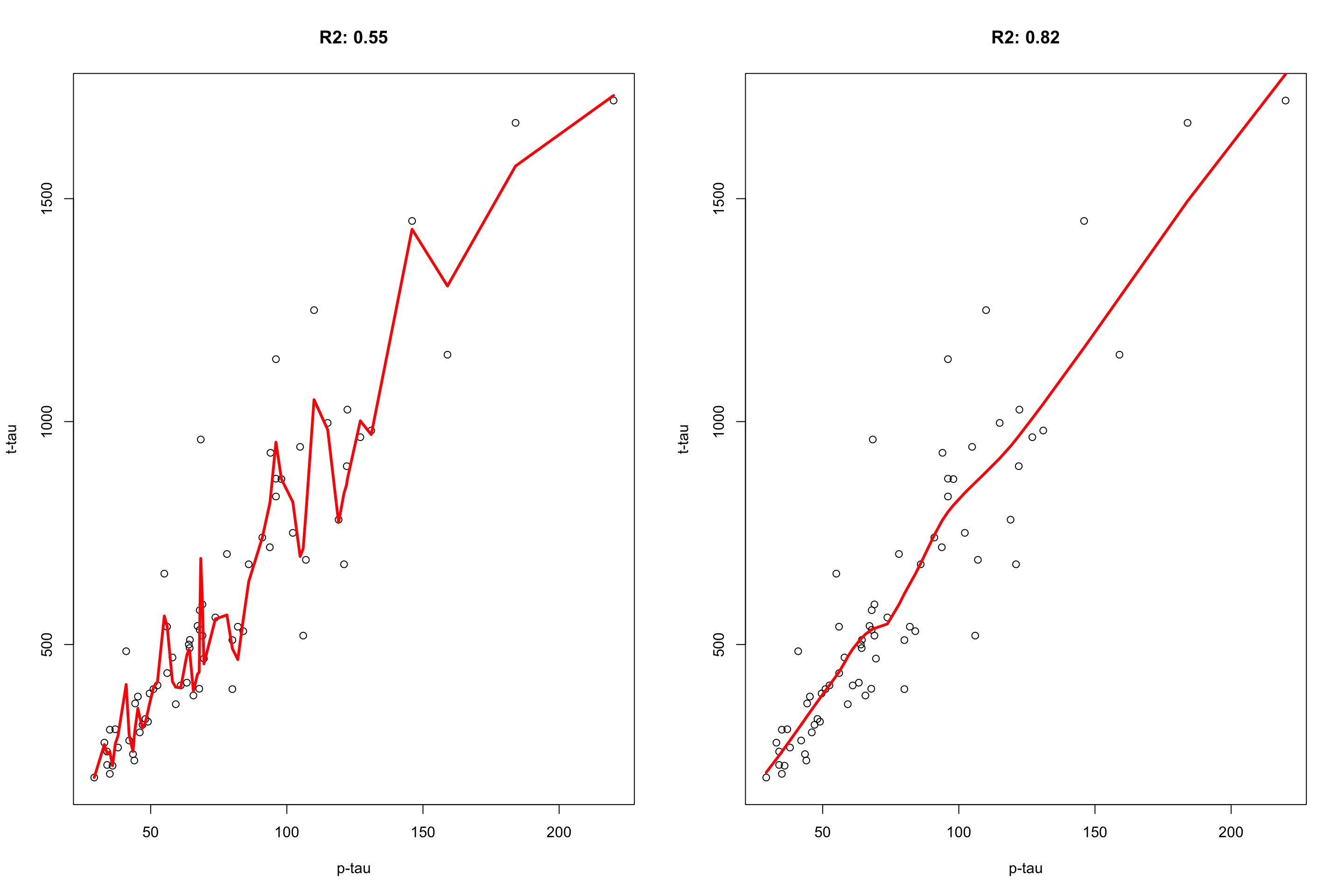
Figure 4.1: plot of p-tau vs t-tau using two models. The model on the left has span of 0.1 and the model on the right has the span of 0.6.
The model on the left fits the training data really good but it performs poorly on the validation set \(R^2=0.55\) whereas the model on the right has a poorer fit on the training data but achieves better performance on the validation set. We tend to say that the model has low bias high variance. That is because it pays too much attention to the training data so that it fails to generalize to what it has not seen before. Decision trees suffer from the same problem. If trained too much, they will have a fantastically low bias but very high variance. The idea behind bagging is to reduce this variance through training multiple models on the same data. Let’s see how it works and why it works.
4.2 Bootstrap aggregating
The idea behind bootstrap aggregating is to subsample the data (with replacement) into different datasets of the same size. These datasets are then independently modelled using for example decision trees. For the prediction, we look at what each of the trees tells us about the value of the new sample and simply accept what the majority of them are saying!
More formally, if we assume that we have \(N\) samples in our datasets we do the following:
Take a random sample of size \(N\) with replacement from the original dataset.
Train a decision tree on this subset (no pruning here. We want this to have a relatively high bias).
Repeat the step 1 and 2 many many times.
Predict each sample to a final group by a majority vote over the set of trees. For example, if we have 500 trees and 400 of them say sample \(x\) is AD, then we use this as the predicted group for the sample \(x\). For regression, we simply take the mean of all the predicted values of all the 500 trees.
Please note that we let each tree to grow reasonably large to capture each tree point of view of our problem. This often leads to high variance in each tree but then we the averaging or the majority of the vote will reduce this variance to a reasonable number. More formally if we define our variance as \(\sigma^2\) for a single variable, having \(m\) variables (independently and identically distributed) will give us \(\frac{\sigma^2}{m}\). In the case of bagging, since we draw from the same pool of samples, we don’t have independently distributed samples so we have to take correlation into account. Thus our variance of average becomes \(p\sigma^2+\frac{1-p}{m}\sigma^2\) where \(p\) is pairwise correlation between different trees and \(\sigma^2\) is the variance. It is easy to see that if we increase \(m\) to a very large number (total number of resampling) we end up have our variance as \(p\sigma^2\). That means that unless we have a perfect correlation between the trees, we will reduce the variance and as the result getting better predictions.
4.3 Out-Of-Bag error
One cool thing about bagging is that it comes with almost a free cross-validation built-in! Remember that when we do resampling, each time, some of our samples will not be selected for modelling. If we do have not too few samples, we can use those samples to estimate what is so-called, out-of-bag error. For example, imagine that we have a dataset with 5 samples (\(x_1,x_2,x_3,x_4,x_5\)) samples. We decide to do decision trees with bagging and 3 resamplings. First we select subsample of the data (\(x_1,x_2,x_2,x_4,x_4\)) and do a decision tree (\(T_1\)). Please note that we did not select \(x_3\) and \(x_5\). We now do another tree (\(T_2\)) and we select these samples to do that: (\(x_1,x_2,x_2,x_2,x_2\)). For the last time, we do \(T_3\) and select (\(x_1,x_2,x_2,x_3,x_4\)). To calculate out of bag error, we look at \(x_3\), we see that we did not use this sample in \(T_1\) and \(T_2\) so we use these two trees to predict the class of this sample. We now look at \(x_4\) and see that we have not used this sample in \(T_2\). We use \(T_2\) to predict \(x_4\). Finally, we see that \(X_5\) has not been used in any of the trees, then we used all the trees to predict \(x_5\). So we have tree samples predicted by the trees that have never seen these samples giving us an estimated cross-validation measure even without doing cross-validation! Given, enough samples, out of bag error will be close to 3-fold cross-validation.
4.4 Application
In R, we can use, ipred together with rpart package to perform bagging.
library(ipred)
library(rpart)
par(mfrow=c(1,2))
set.seed(20)
testing_index<-sample(1:length(data$p_tau),100,replace = F)

limited_data4_training<-data[-testing_index,]
limited_data4_testing<-data[testing_index,]

limited_data4_training$group<-as.factor(limited_data4_training$group)
limited_data4_training$gender<-as.factor(limited_data4_training$gender)

limited_data4_testing$group<-as.factor(limited_data4_testing$group)
limited_data4_testing$gender<-as.factor(limited_data4_testing$gender)

set.seed(10)
bagged_model <- bagging(group ~ ., data = limited_data4_training,nbagg=100)


set.seed(10)
tree_model <- rpart(group ~ ., data = limited_data4_training,
   method="class")
set.seed(10)
tree_model<- prune(tree_model, cp=   tree_model$cptable[which.min(tree_model$cptable[,"xerror"]),"CP"])

acc_bagging<-mean(limited_data4_testing$group == predict(bagged_model,limited_data4_testing,type = "class"))

acc_tree<-mean(limited_data4_testing$group == predict(tree_model,limited_data4_testing,type = "class"))


confMatrix_bagging<-caret::confusionMatrix(predict(bagged_model,limited_data4_testing[,-7],type = "class"),limited_data4_testing$group )
confMatrix_tree<-caret::confusionMatrix(predict(tree_model,limited_data4_testing[,-7],type = "class"),limited_data4_testing$group )


plot_data<-rbind(data.frame(reshape::melt(confMatrix_bagging$table),Method="Bagging"),
      data.frame(reshape::melt(confMatrix_tree$table),Method="Normal"))

names(plot_data)[1:2]<-c("x","y")
plot_data$Color=NA
plot_data$Color[plot_data$x==plot_data$y]<-"red"
library(ggplot2)

ggplot(plot_data, aes(Method,fill=Method)) +
    geom_bar(aes(y = value),
             stat = "identity"#, position = "dodge"
             ) +
    geom_text(aes(y = -5, label = value,color=Method)) +
    facet_grid(x ~ y, switch = "y") +
    labs(title = "",
         y = "Predicted class",
         x = "True class") +
    theme_bw() +
   geom_rect(data=plot_data, aes(fill=Color), xmin=-Inf, xmax=Inf, ymin=-Inf, ymax=Inf, alpha=0.095)+
  scale_fill_manual(values=c("blue", "red","red"), breaks=NULL)+
    scale_color_manual(values=c("blue", "red"), breaks=NULL)+
    theme(strip.background = element_blank(),panel.border = element_rect(color = , fill = NA, size = 1),
          axis.text.y = element_blank(),
          axis.text.x = element_text(size = 9),
          axis.ticks = element_blank(),
          strip.text.y = element_text(angle = 0),
          strip.text = element_text(size = 9))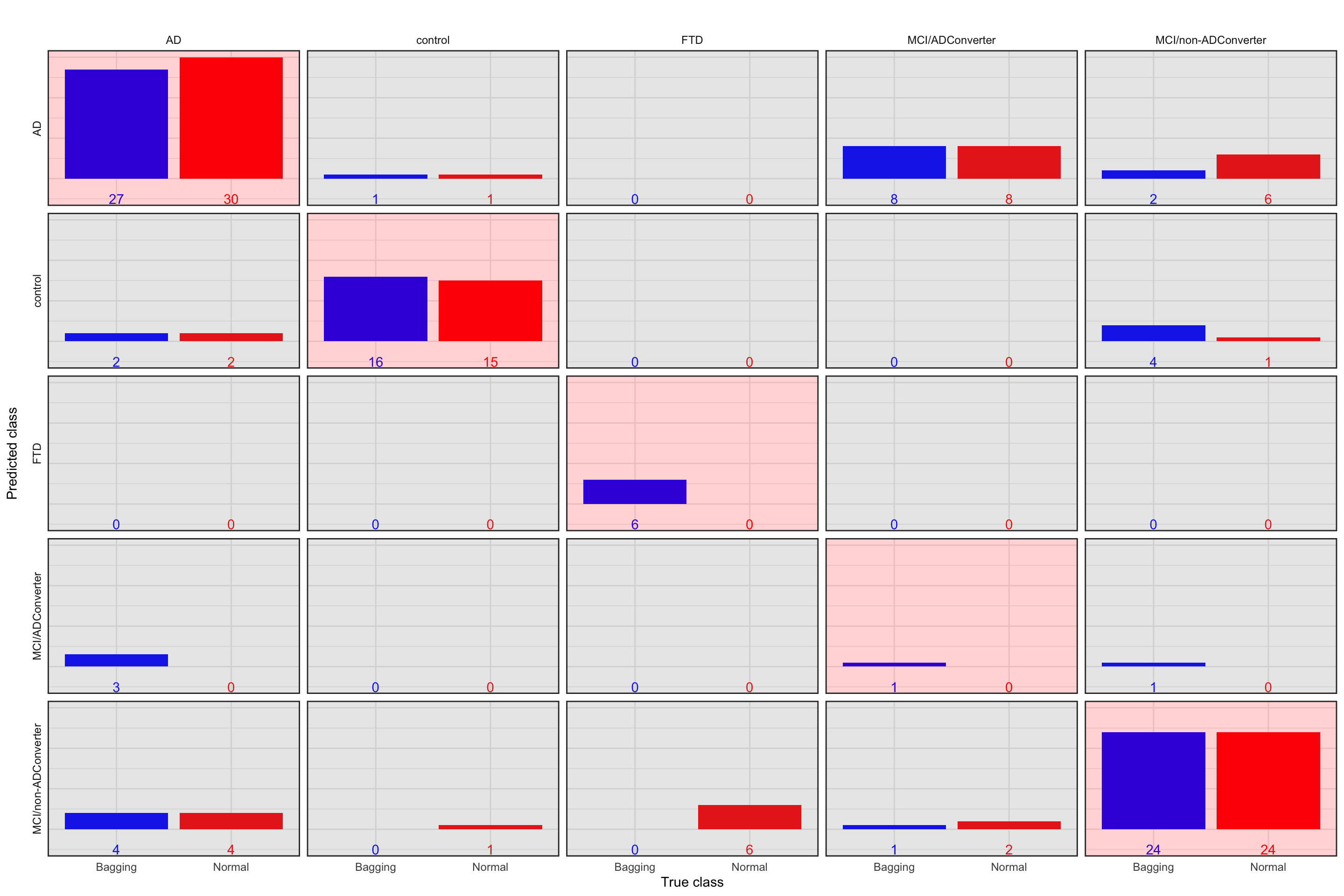
Figure 4.2: Prediction accuracy of normal tree vs. bagging. Blue bar: Bagging, red bar: Normal. The plots with red background are correct classification
The above plot shows the performance of both models in classification. The observed (true) classes of predicted samples are on \(x\) axis and the predicted class are on \(y\) axis. Let’s give one example to clarify how to interpret this plot. We take the first column which is for samples with classes of AD. We see that bagging classified 27 correctly to AD whereas the normal tree has assigned 30 to AD. Both of these methods have assigned two of the AD samples wrongly to control. No samples have been classified as FTD. Bagging has wrongly predicted 3 AD to be MCI/ADConverter and finally both these methods wrongly predicted 4 AD to be MCI/non-ADConverter. Similarly, we can interpret the other columns. In general, we have the accuracy of 0.69 for the normal tree and the accuracy of 0.74 for bagging. Bagging performs a bit better. One interesting observation here is the MCI/ADConverter. These samples are persons who were suspected to have AD but they did not show the molecular signature at the time of sampling. However, later on, these samples were diagnosed to have AD. Interestingly, our models assign 8 of these samples as AD so correctly predicting the future without even knowing about it!
That was it for bagging. I guess we already noticed that simply doing bootstrapping does not ensure we significantly reduce the variance. Random forest will try to address this problem.