SOM Practice in Python

In this practical we will train a self-organizing map on miRNA measurements from 220 breast cancer samples. Each sample has 184 features and one known subtype: Basal, Her2, or Luminal A. The subtype is kept out of the training data and added later to help us interpret the map.

We will use TorchSOM. It provides the SOM model and the main plots we need, including hit maps, U-matrices, training curves, classification maps, and component planes.

pip install torchsom pandas scikit-learn "matplotlib<3.10"

The Matplotlib upper bound avoids a plotting API incompatibility in TorchSOM 1.3.0.

Prepare the data

Download breast_tcga_mirna.csv and keep it in a data folder next to your script.

import pandas as pd
import torch
from sklearn.preprocessing import StandardScaler
from torchsom import SOM, SOMVisualizer

torch.set_num_threads(1)

df = pd.read_csv("data/breast_tcga_mirna.csv")
feature_cols = [
    column for column in df.columns
    if column not in ("sample_id", "subtype")
]

scaler = StandardScaler()
X_scaled = scaler.fit_transform(df[feature_cols]).astype("float32")
X = torch.tensor(X_scaled)

subtype_code, subtype_names = pd.factorize(df["subtype"], sort=True)
# TorchSOM uses zero as the plot background, so class labels start at 1.
y = torch.tensor(subtype_code + 1)

print(X.shape)
print(df["subtype"].value_counts())

torch.Size([220, 184])
subtype
LumA     110
Basal     66
Her2      44
Name: count, dtype: int64

SOM training uses distances, so features with a large variance can dominate the map. Standardization puts every miRNA on a comparable scale. In a predictive study, the scaler must be fitted on the training set and then applied to the test set. Here we are doing one exploratory analysis of the full dataset.

Train the map

The map below has 25 units arranged on a hexagonal grid. PCA initialization gives the units an ordered starting position and the random seed makes the remaining stochastic steps reproducible.

som = SOM(
    x=5,
    y=5,
    num_features=X.shape[1],
    epochs=100,
    batch_size=16,
    sigma=1.5,
    learning_rate=0.5,
    topology="hexagonal",
    initialization_mode="pca",
    device="cpu",
    random_seed=101,
    search_backend="torch",
)

som.initialize_weights(data=X, mode="pca")
qe_history, te_history = som.fit(data=X)

An epoch is one pass through the samples. Early updates organize broad regions of the grid. Later updates make smaller local adjustments as the learning rate and neighborhood width decrease.

viz = SOMVisualizer(som)
viz.plot_training_errors(qe_history, te_history)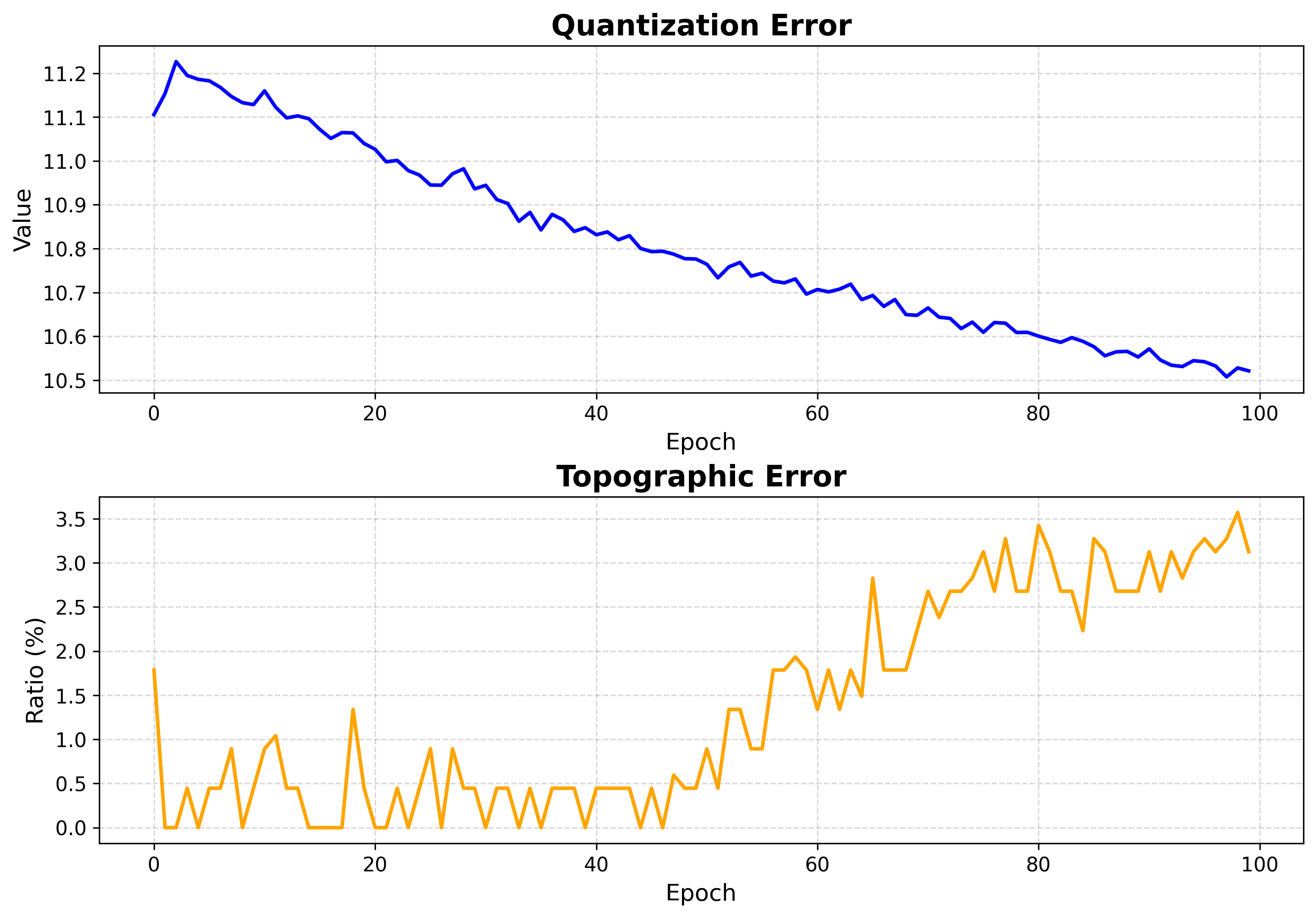

Figure 2.1: Training diagnostics for the 100 epochs. Quantization error decreases overall. Topographic error remains low but fluctuates because it is calculated within training batches.

The declining quantization error shows that the prototypes are moving closer to the samples. A perfectly smooth curve is not expected because the sample order changes between epochs.

Assign samples to units

Each sample is assigned to its best matching unit, or BMU. A BMU is the unit whose prototype vector is closest to that sample.

bmus = som.identify_bmus(X).cpu().numpy()

bmu_table = pd.DataFrame({
    "sample_id": df["sample_id"],
    "subtype": df["subtype"],
    "bmu_row": bmus[:, 0],
    "bmu_col": bmus[:, 1],
})
print(bmu_table.head())

  sample_id subtype  bmu_row  bmu_col
0      A0FJ   Basal        4        4
1      A13E   Basal        3        3
2      A0G0   Basal        4        3
3      A0SX   Basal        4        1
4      A143   Basal        3        3

Several samples can share a BMU. The hit map shows how many samples are assigned to each unit.

viz.plot_hit_map(data=X)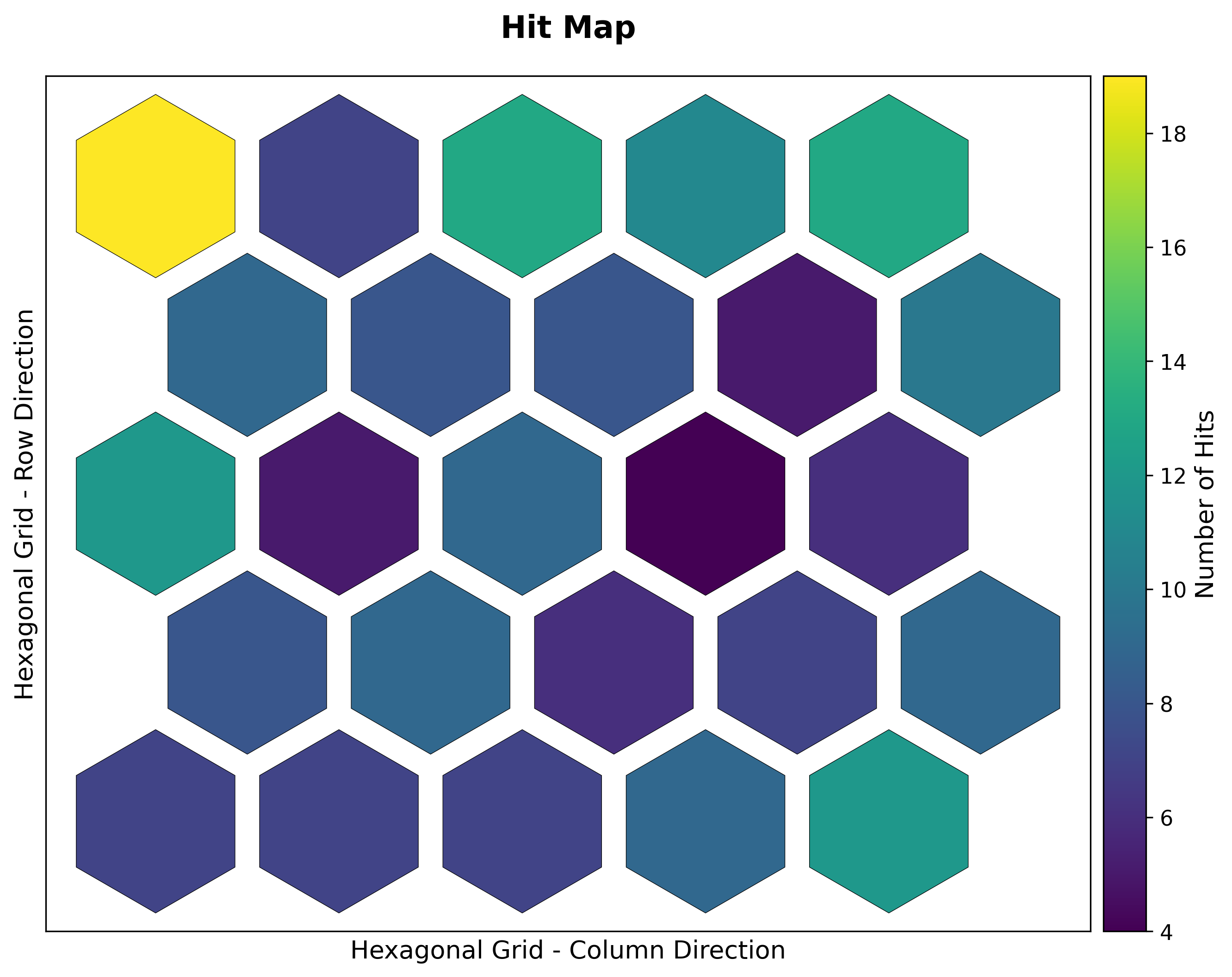

Figure 2.2: Number of samples assigned to each SOM unit.

All 25 units are occupied. Counts range from 4 to 19, so no prototype is unused, although the allocation is not perfectly even. An uneven hit map is not automatically a problem. It often reflects uneven density in the original data.

Check map quality

qe = som.quantization_error(X)
te = som.topographic_error(X)

print(f"quantization error: {qe:.4f}")
print(f"topographic error:  {te:.4f}")

quantization error: 10.5675
topographic error:  0.0364

The quantization error is the mean distance from a sample to its BMU prototype. Its value depends on the feature scale and the number of features, so there is no universal cutoff for a good result. It is most useful when comparing candidate maps fitted to the same transformed data.

The topographic error is the proportion of samples whose two closest units are not neighbors. Here it is about 3.6%, which means that local ordering is preserved for most samples. The two diagnostics answer different questions. A map can represent samples closely while arranging its prototypes poorly, or preserve topology while using overly smooth prototypes.

Add the subtype labels

The subtype labels were not used during fitting. The classification map colors each occupied unit by its most common subtype.

bmu_index = som.build_map(
    "bmus_data",
    data=X,
    return_indices=True,
)

viz.plot_classification_map(
    bmus_data_map=bmu_index,
    data=X,
    target=y,
)

print(dict(enumerate(subtype_names, start=1)))

{1: 'Basal', 2: 'Her2', 3: 'LumA'}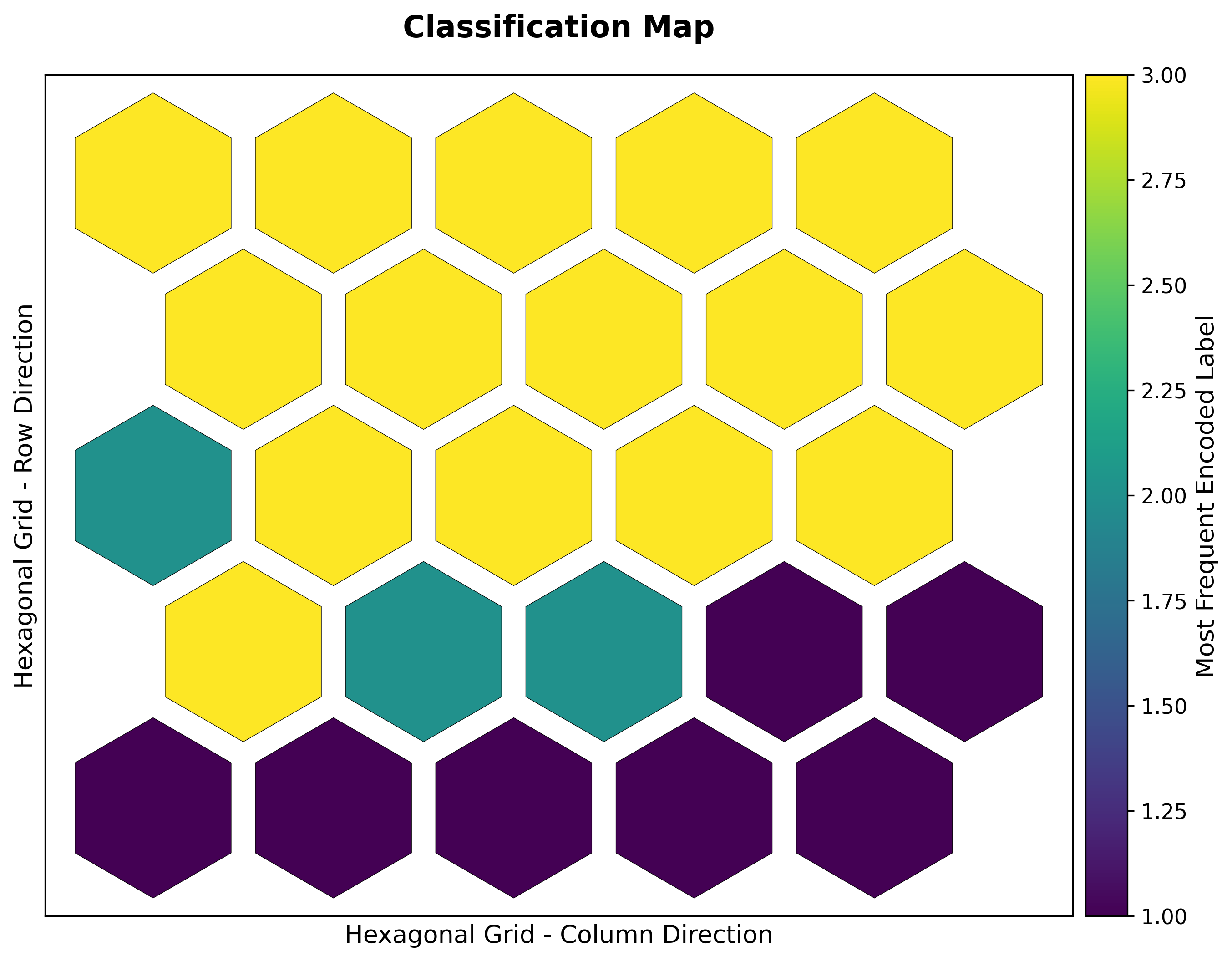

Figure 2.3: Majority subtype in each occupied unit. The numeric labels are Basal = 1, Her2 = 2, and Luminal A = 3.

Luminal A dominates the upper part of the map and Basal dominates the lower part. Her2 appears mainly between those regions. This suggests a gradual change in expression profiles rather than three isolated blocks.

The plot shows only the majority label in each unit. It does not show purity, uncertainty, or predictive accuracy. A cross-tabulation is needed before making stronger claims.

unit_id = bmus[:, 0] * som.y + bmus[:, 1]
print(pd.crosstab(unit_id, df["subtype"]))

Many units contain more than one subtype. The label map is therefore a compact summary of a mixed pattern, not a supervised classification result.

Read the U-matrix

The U-matrix summarizes how different each prototype is from its immediate neighbors.

viz.plot_distance_map(
    distance_metric="euclidean",
    neighborhood_order=1,
    scaling="mean",
)

Figure 2.4: U-matrix for the fitted SOM.

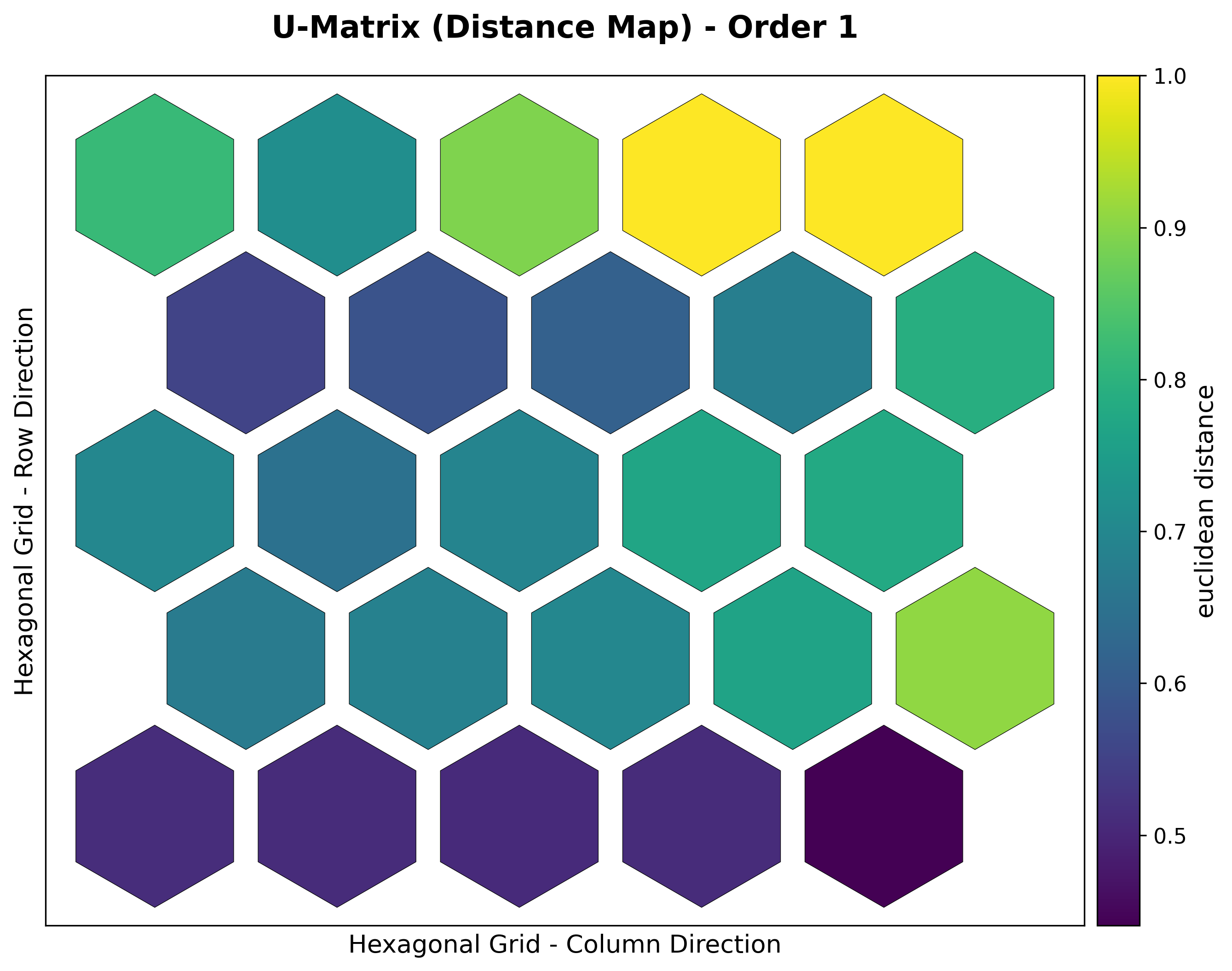
Bright units have prototypes that differ more from their neighbors. Dark units sit in smoother regions. A bright ridge can suggest a boundary worth investigating, but it is not a statistical test and does not determine the number of clusters.

Inspect individual miRNAs

Every unit has a prototype value for each of the 184 miRNAs. A component plane displays one feature across the same grid.

for feature in ["hsa-mir-130b", "hsa-mir-17"]:
    feature_index = feature_cols.index(feature)
    viz.plot_grid(
        map=som.weights[:, :, feature_index],
        title=f"Component plane: {feature}",
        colorbar_label="standardized prototype value",
        filename=feature,
        cmap="coolwarm",
        mask_zeros=False,
    )

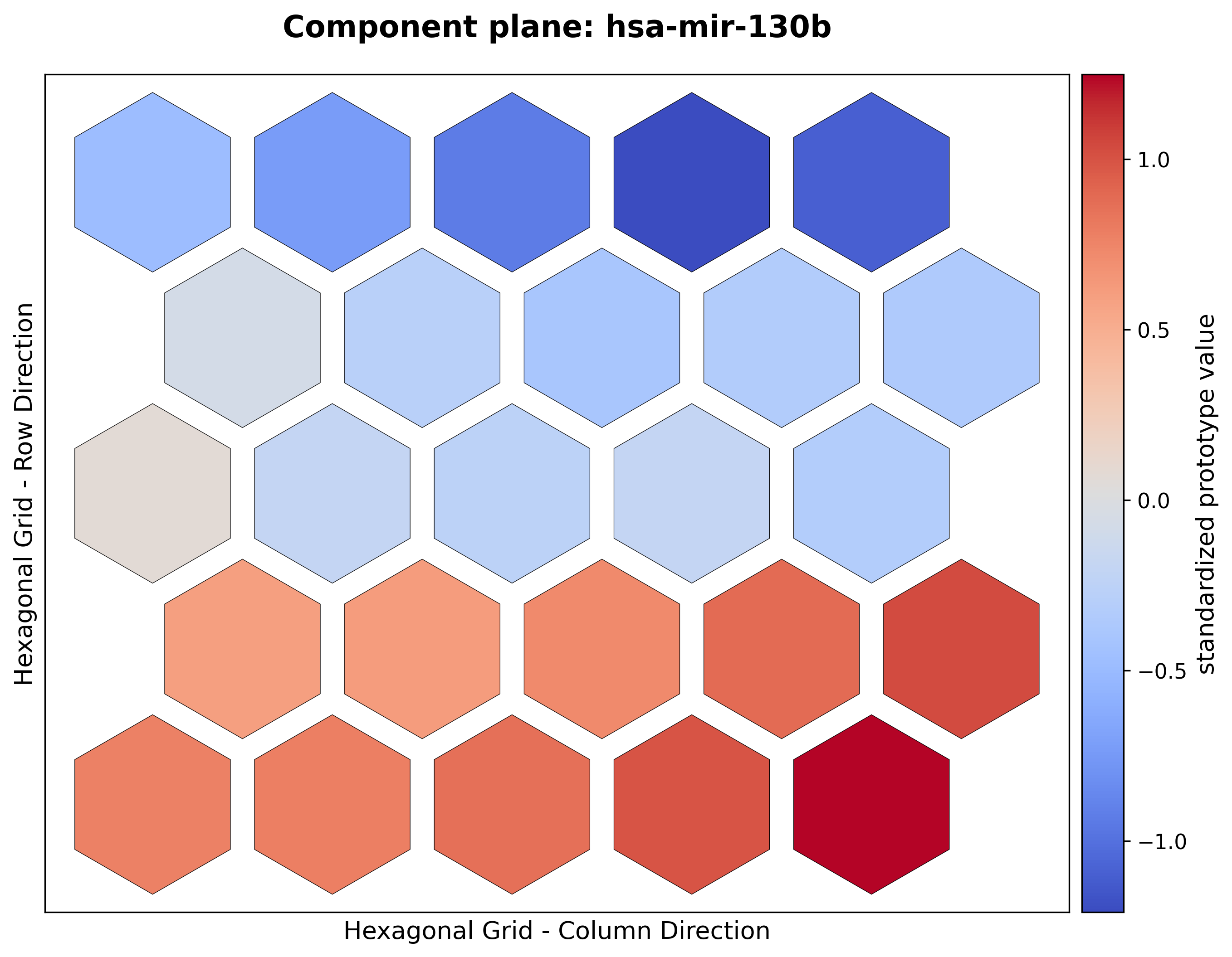
Figure 2.5: Component plane for hsa-mir-130b.

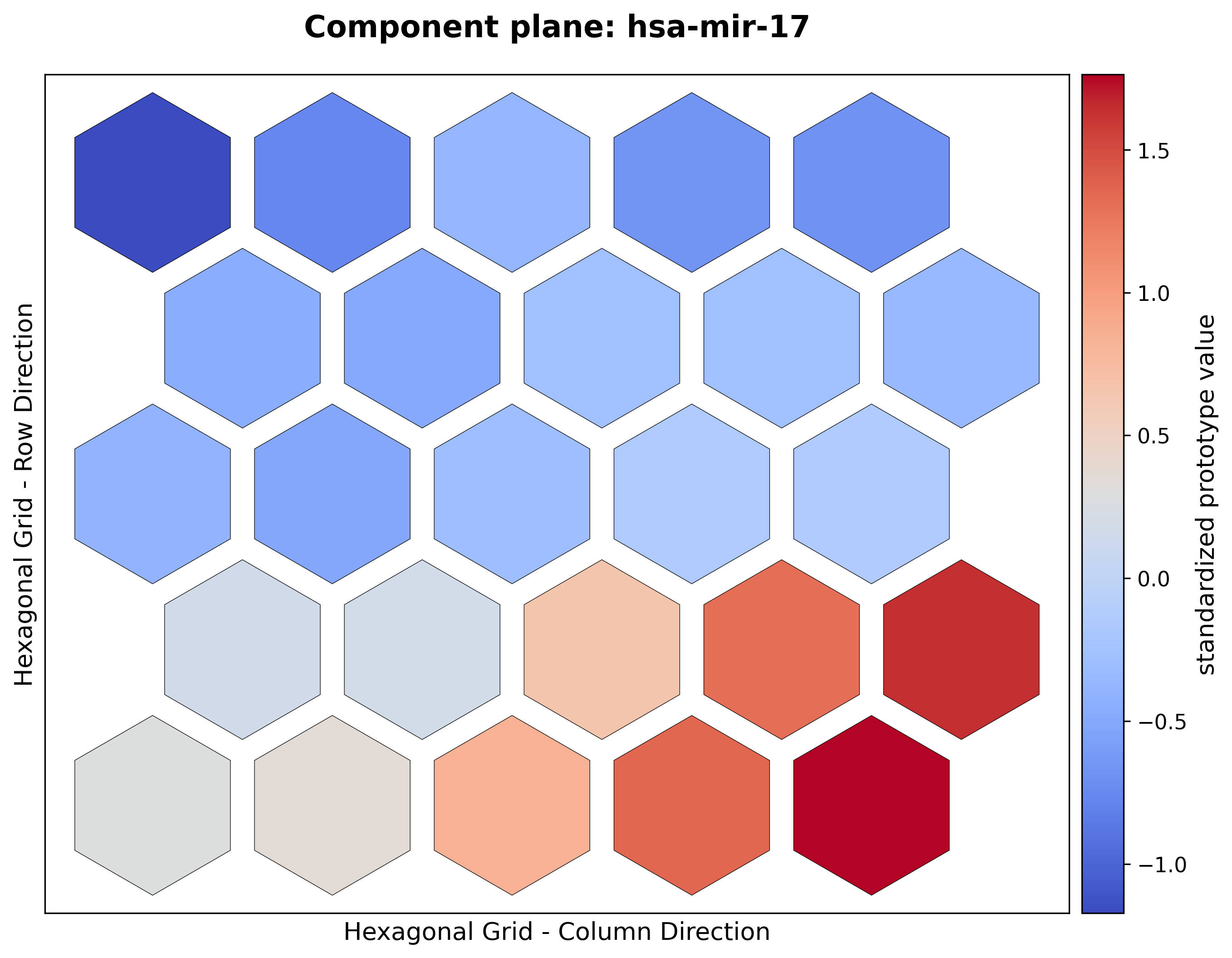
Figure 2.6: Component plane for hsa-mir-17.

Both miRNAs are low in the Luminal A region and high in the Basal region. This agrees with their observed subtype means in the original data. The two planes are similar but not identical, which indicates related rather than interchangeable expression patterns.

Component planes are often the most useful part of a SOM analysis. They connect the geometry of the map back to named biological measurements.