SOM Exercises

These exercises use hepatic fatty acid measurements from 40 mice. The mice belong to two genotypes and received one of five diets. The SOM sees only the 21 fatty acid measurements. Genotype and diet are kept for interpretation after training.

Download nutrimouse_lipids.csv and keep it in a data folder next to your script.

Solutions are provided in R and Python. Treat the numerical output as implementation-specific and interpret it within that workflow.

Setup

R

library(kohonen)

df <- read.csv("data/nutrimouse_lipids.csv")
feature_cols <- setdiff(
  names(df),
  c("sample_id", "genotype", "diet")
)

X_raw <- as.matrix(df[, feature_cols])
X_scaled <- scale(X_raw)
genotype <- factor(df$genotype)

topographic_error <- function(model, values) {
  prototypes <- model$codes[[1]]
  all_distances <- as.matrix(dist(rbind(values, prototypes)))
  n_samples <- nrow(values)
  grid_distances <- as.matrix(unit.distances(model$grid))

  errors <- sapply(seq_len(n_samples), function(i) {
    nearest <- order(
      all_distances[i, n_samples + seq_len(nrow(prototypes))]
    )[1:2]
    grid_distances[nearest[1], nearest[2]] > 1.01
  })
  mean(errors)
}

fit_som <- function(
    values,
    grid = c(5, 5),
    radius = 1.5,
    rlen = 100,
    seed = 101) {
  som_grid <- somgrid(
    xdim = grid[1],
    ydim = grid[2],
    topo = "hexagonal",
    neighbourhood.fct = "gaussian"
  )

  set.seed(seed)
  model <- som(
    X = values,
    grid = som_grid,
    rlen = rlen,
    alpha = c(0.05, 0.01),
    radius = radius,
    keep.data = TRUE
  )

  list(
    model = model,
    qe = mean(sqrt(model$distances)),
    te = topographic_error(model, values),
    occupied = length(unique(model$unit.classif))
  )
}

Python

import numpy as np
import pandas as pd
import torch
from sklearn.preprocessing import StandardScaler
from torchsom import SOM, SOMVisualizer

torch.set_num_threads(1)

df = pd.read_csv("data/nutrimouse_lipids.csv")
feature_cols = [
    column for column in df.columns
    if column not in ("sample_id", "genotype", "diet")
]

X_raw = df[feature_cols].to_numpy(dtype="float32")
X_scaled = StandardScaler().fit_transform(X_raw).astype("float32")


def fit_som(
    values,
    grid=(5, 5),
    sigma=1.5,
    epochs=100,
    seed=101,
):
    data = torch.tensor(values)
    som = SOM(
        x=grid[0],
        y=grid[1],
        num_features=data.shape[1],
        epochs=epochs,
        batch_size=8,
        sigma=sigma,
        learning_rate=0.5,
        topology="hexagonal",
        initialization_mode="pca",
        device="cpu",
        random_seed=seed,
        search_backend="torch",
    )
    som.initialize_weights(data=data, mode="pca")
    qe_history, te_history = som.fit(data=data, verbose=False)
    bmus = som.identify_bmus(data).cpu().numpy()

    return {
        "som": som,
        "data": data,
        "bmus": bmus,
        "qe": som.quantization_error(data),
        "te": som.topographic_error(data),
        "occupied": len(np.unique(bmus, axis=0)),
        "qe_history": qe_history,
        "te_history": te_history,
    }

The helper in each language keeps all settings fixed unless an exercise changes one of them.

Exercise 1. Should the fatty acids be standardized?

Inspect the standard deviation of each fatty acid. Then fit one SOM to the raw percentages and another to standardized values. What changes, and which quantities can be compared fairly?

NoteSolution

R

feature_sd <- sort(apply(X_raw, 2, sd))
print(feature_sd[c(1, length(feature_sd))])
cat("ratio:", max(feature_sd) / min(feature_sd), "\n")

raw_fit <- fit_som(X_raw)
scaled_fit <- fit_som(X_scaled)

cat(
  "raw   ",
  raw_fit$qe,
  raw_fit$te,
  raw_fit$occupied,
  "\n"
)
cat(
  "scaled",
  scaled_fit$qe,
  scaled_fit$te,
  scaled_fit$occupied,
  "\n"
)

C20.1n.9  C18.2n.6
    0.140      8.760
ratio: 62.7

raw    3.128 0.000 15
scaled 1.115 0.050 15

Python

feature_sd = pd.Series(
    X_raw.std(axis=0, ddof=1),
    index=feature_cols,
).sort_values()

print(feature_sd.iloc[[0, -1]])
print("ratio:", feature_sd.iloc[-1] / feature_sd.iloc[0])

raw_fit = fit_som(X_raw)
scaled_fit = fit_som(X_scaled)

for name, result in [("raw", raw_fit), ("scaled", scaled_fit)]:
    print(
        name,
        f"QE={result['qe']:.3f}",
        f"TE={result['te']:.3f}",
        f"occupied={result['occupied']}/25",
    )

C20.1n.9    0.140
C18.2n.6    8.760
dtype: float32
ratio: 62.7

raw    QE=3.674 TE=0.025 occupied=15/25
scaled QE=1.214 TE=0.000 occupied=16/25

The most variable fatty acid has about 63 times the standard deviation of the least variable one. Without standardization, it has far more influence on Euclidean distance and therefore on BMU selection.

Do not compare the raw and standardized quantization errors directly. Standardization changes the units of distance, so the two errors are on different scales. Topographic error and occupancy remain meaningful summaries.

Standardization gives relative differences in each fatty acid similar influence. It does not solve the special geometry of compositional data. For a dedicated compositional analysis, a suitable log-ratio transformation should also be considered.

Exercise 2. How large should the grid be?

Fit 3 by 3, 5 by 5, and 6 by 6 maps to the standardized data. Compare quantization error, topographic error, and the number of empty units.

NoteSolution

R

for (grid in list(c(3, 3), c(5, 5), c(6, 6))) {
  result <- fit_som(X_scaled, grid = grid)
  units <- prod(grid)
  empty <- units - result$occupied
  cat(
    paste0(grid[1], "x", grid[2]),
    sprintf("QE=%.3f", result$qe),
    sprintf("TE=%.3f", result$te),
    sprintf("empty=%d/%d", empty, units),
    "\n"
  )
}

3x3 QE=2.004 TE=0.025 empty=0/9
5x5 QE=1.115 TE=0.050 empty=10/25
6x6 QE=0.925 TE=0.100 empty=19/36

Python

for grid in [(3, 3), (5, 5), (6, 6)]:
    result = fit_som(X_scaled, grid=grid)
    units = grid[0] * grid[1]
    empty = units - result["occupied"]
    print(
        f"{grid[0]}x{grid[1]}",
        f"QE={result['qe']:.3f}",
        f"TE={result['te']:.3f}",
        f"empty={empty}/{units}",
    )

3x3 QE=2.409 TE=0.000 empty=1/9
5x5 QE=1.214 TE=0.000 empty=9/25
6x6 QE=0.977 TE=0.025 empty=18/36

Quantization error falls as the grid grows because a larger map has more prototypes. That alone does not make the largest grid the best choice. Empty units rise sharply, and topographic error can also increase.

For 40 samples, a 5 by 5 grid is a reasonable compromise. It gives more detail than the 3 by 3 map without leaving half the grid unused. Grid size controls resolution, not the number of biological groups.

Exercise 3. What does the neighborhood width control?

Fit the 5 by 5 map using several neighborhood widths. In R, vary radius. In Python, vary sigma. Look for a trade-off between quantization error and topographic error.

NoteSolution

R

radii <- c(0.5, 1.0, 1.5, 2.0, 3.0)
radius_results <- data.frame(radius = radii, qe = NA, te = NA)

for (i in seq_along(radii)) {
  result <- fit_som(X_scaled, radius = radii[i])
  radius_results$qe[i] <- result$qe
  radius_results$te[i] <- result$te
  cat(
    sprintf("radius=%.1f", radii[i]),
    sprintf("QE=%.3f", result$qe),
    sprintf("TE=%.3f", result$te),
    "\n"
  )
}

radius=0.5 QE=1.317 TE=0.225
radius=1.0 QE=1.317 TE=0.225
radius=1.5 QE=1.115 TE=0.050
radius=2.0 QE=1.194 TE=0.000
radius=3.0 QE=1.339 TE=0.000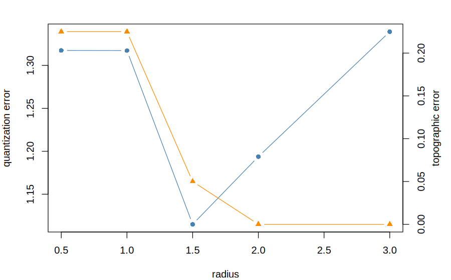

Figure 3.1: Quantization and topographic error across neighborhood radii in R.

Python

sigma_results = []

for sigma in [0.5, 1.0, 1.5, 2.0, 3.0]:
    result = fit_som(X_scaled, sigma=sigma)
    sigma_results.append((sigma, result["qe"], result["te"]))
    print(
        f"sigma={sigma:.1f}",
        f"QE={result['qe']:.3f}",
        f"TE={result['te']:.3f}",
    )

sigma=0.5 QE=0.879 TE=0.075
sigma=1.0 QE=0.984 TE=0.050
sigma=1.5 QE=1.214 TE=0.000
sigma=2.0 QE=1.598 TE=0.000
sigma=3.0 QE=2.339 TE=0.000

import matplotlib.pyplot as plt

result_table = pd.DataFrame(
    sigma_results,
    columns=["sigma", "quantization_error", "topographic_error"],
)

fig, ax1 = plt.subplots(figsize=(6, 4))
ax1.plot(
    result_table["sigma"],
    result_table["quantization_error"],
    marker="o",
    color="steelblue",
)
ax1.set_xlabel("sigma")
ax1.set_ylabel("quantization error", color="steelblue")

ax2 = ax1.twinx()
ax2.plot(
    result_table["sigma"],
    result_table["topographic_error"],
    marker="o",
    color="darkorange",
)
ax2.set_ylabel("topographic error", color="darkorange")
plt.show()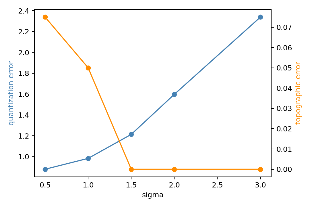

Figure 3.2: Quantization and topographic error across neighborhood widths in Python.

A narrow neighborhood allows prototypes to specialize, which can lower quantization error at the cost of poorer ordering. A broad neighborhood keeps the map orderly but can make prototypes too similar. A width near 1.5 gives a useful balance for this dataset. It is not a universal default.

Interpret the selected map

We will use the 5 by 5 standardized fit with neighborhood width 1.5.

R

final_fit <- fit_som(
  X_scaled,
  grid = c(5, 5),
  radius = 1.5
)
model <- final_fit$model

plot(
  model,
  type = "count",
  shape = "straight",
  main = "Samples per SOM unit"
)
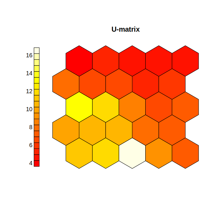
plot(
  model,
  type = "dist.neighbours",
  shape = "straight",
  main = "U-matrix"
)

Figure 3.3: Samples assigned to each unit in the selected R map.

Figure 3.4: U-matrix for the selected R map.

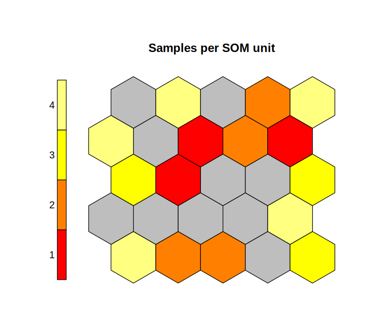
Fifteen units are occupied and ten are empty. Occupied units contain between one and four mice.

Python

final_fit = fit_som(X_scaled, grid=(5, 5), sigma=1.5)
som = final_fit["som"]
X = final_fit["data"]
bmus = final_fit["bmus"]
viz = SOMVisualizer(som)

viz.plot_hit_map(data=X)
viz.plot_distance_map(scaling="mean")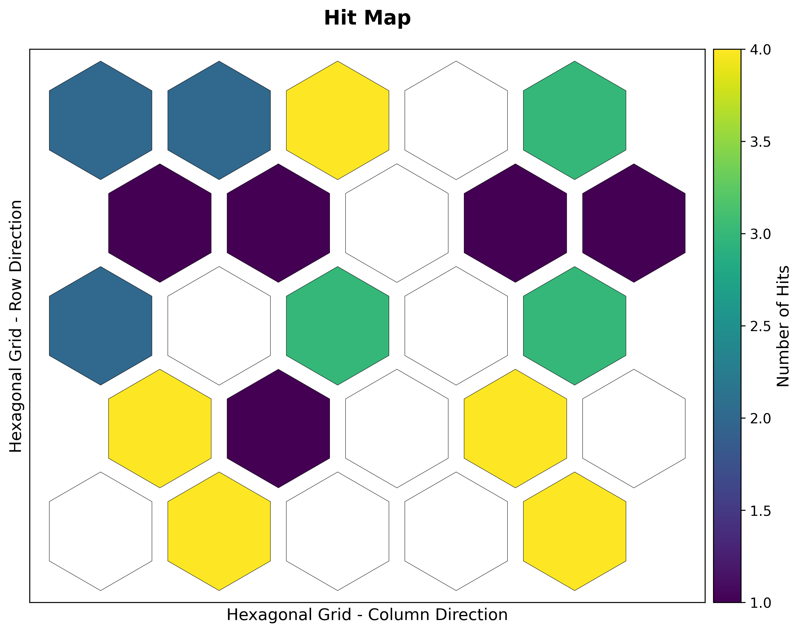

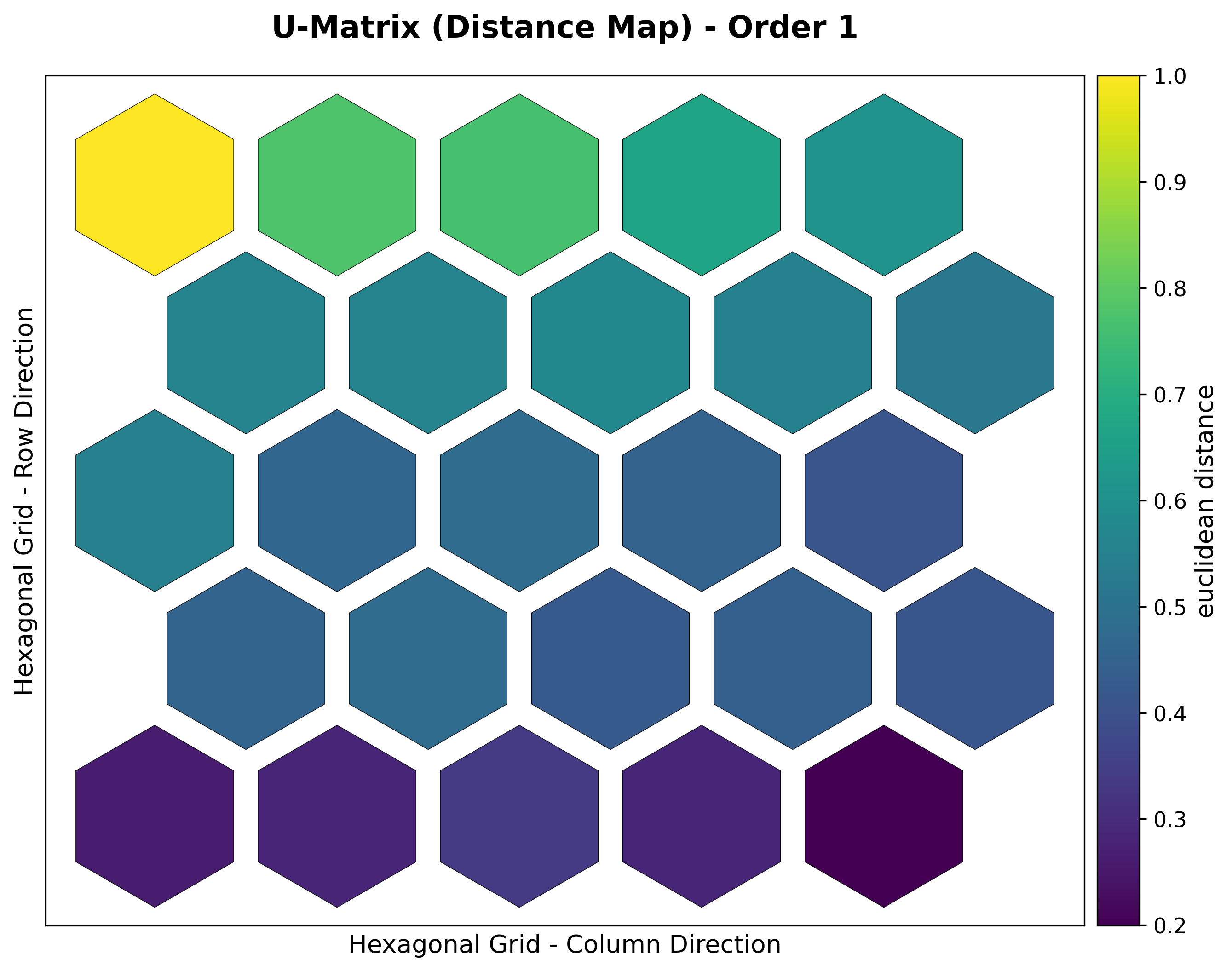
Figure 3.5: Samples assigned to each unit in the selected Python map.

Figure 3.6: U-matrix for the selected Python map.

Sixteen units are occupied and nine are empty. Occupied units contain between one and four mice.

An empty unit is a prototype that is not the closest unit for any observed mouse. It is not automatically a failed cluster. The U-matrix highlights regions where neighboring prototypes differ, but it does not establish cluster boundaries on its own.

Add genotype after training

R

genotype_colors <- setNames(
  c("darkorange", "darkslateblue"),
  levels(genotype)
)

plot(
  model,
  type = "mapping",
  pchs = 16,
  col = genotype_colors[genotype],
  shape = "straight",
  main = "SOM mapping by genotype"
)

unit_table <- table(model$unit.classif, genotype)
sum(apply(unit_table, 1, function(row) sum(row > 0) > 1))

[1] 0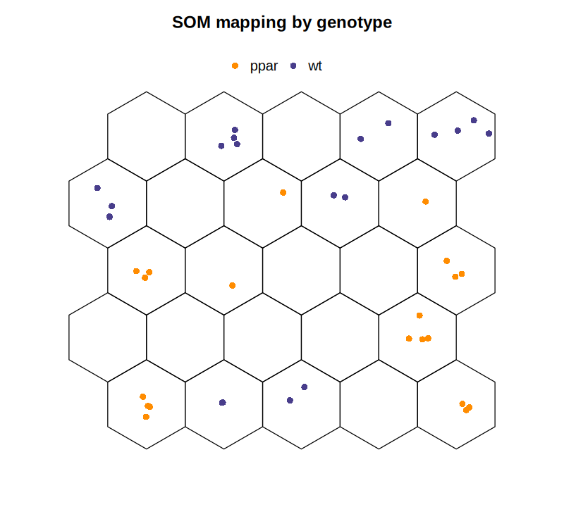

Figure 3.7: Mice mapped to their winning R units and colored by genotype.

Python

genotype_code, genotype_names = pd.factorize(
    df["genotype"],
    sort=True,
)
bmu_index = som.build_map(
    "bmus_data",
    data=X,
    return_indices=True,
)

# TorchSOM uses zero as the plot background, so labels start at 1.
viz.plot_classification_map(
    bmus_data_map=bmu_index,
    data=X,
    target=torch.tensor(genotype_code + 1),
)

unit_id = bmus[:, 0] * som.y + bmus[:, 1]
unit_table = pd.crosstab(unit_id, df["genotype"])
print(((unit_table > 0).sum(axis=1) > 1).sum())
print(dict(enumerate(genotype_names, start=1)))

0
{1: 'ppar', 2: 'wt'}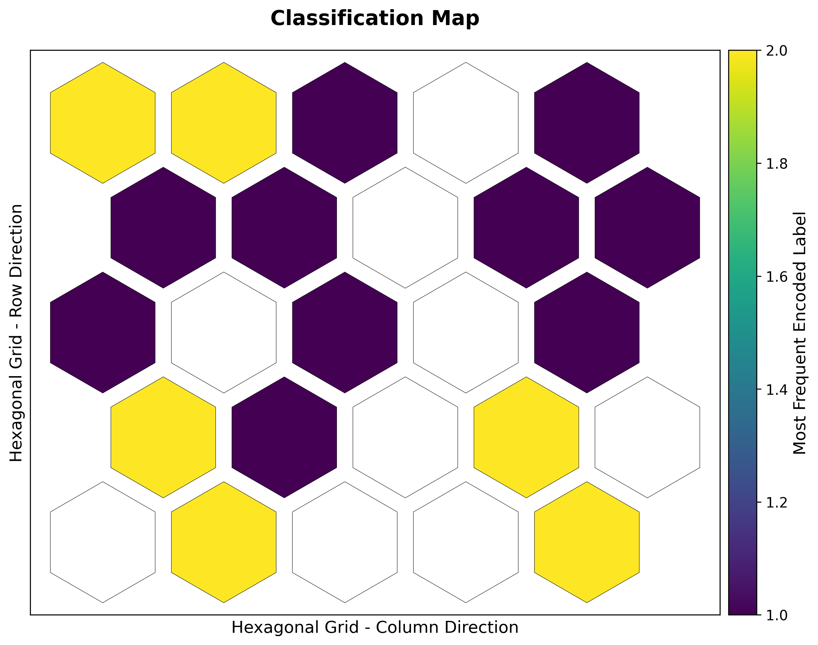

Figure 3.8: Majority genotype in each occupied Python unit. White units are empty.

No occupied unit contains both genotypes in either selected fit. This is evidence that genotype is associated with local fatty acid profiles. It is not an estimate of classification accuracy because the same samples were used to train and inspect the map. It also does not guarantee that each genotype forms one contiguous region.

Inspect two fatty acids

R

for (feature in c("C18.2n.6", "C20.1n.9")) {
  plot(
    model,
    type = "property",
    property = model$codes[[1]][, feature],
    shape = "straight",
    main = paste("Component plane:", feature)
  )
}

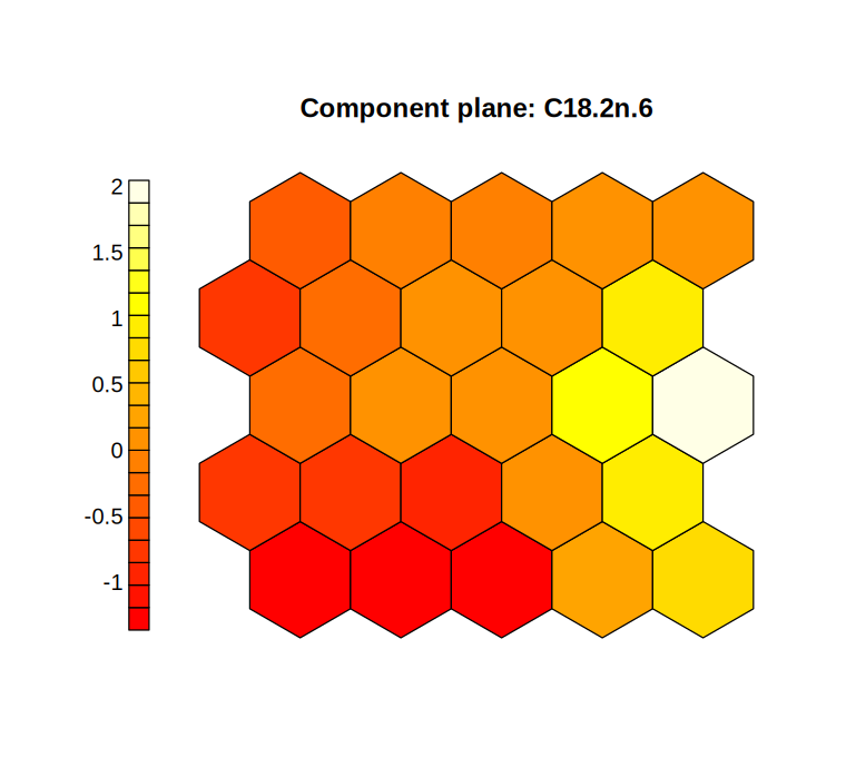
Figure 3.9: R component plane for C18.2n.6.

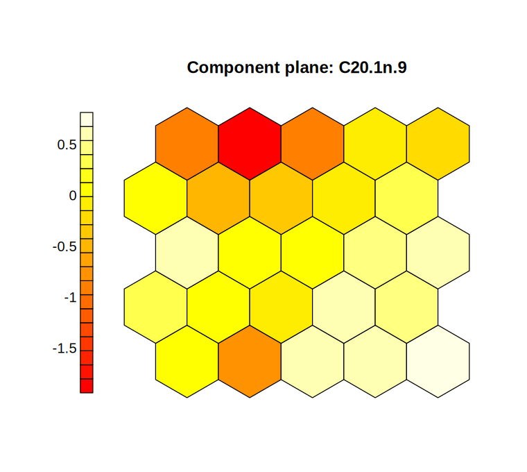
Figure 3.10: R component plane for C20.1n.9.

Python

for feature in ["C18.2n.6", "C20.1n.9"]:
    feature_index = feature_cols.index(feature)
    viz.plot_grid(
        map=som.weights[:, :, feature_index],
        title=f"Component plane: {feature}",
        colorbar_label="standardized prototype value",
        filename=feature,
        cmap="coolwarm",
        mask_zeros=False,
    )

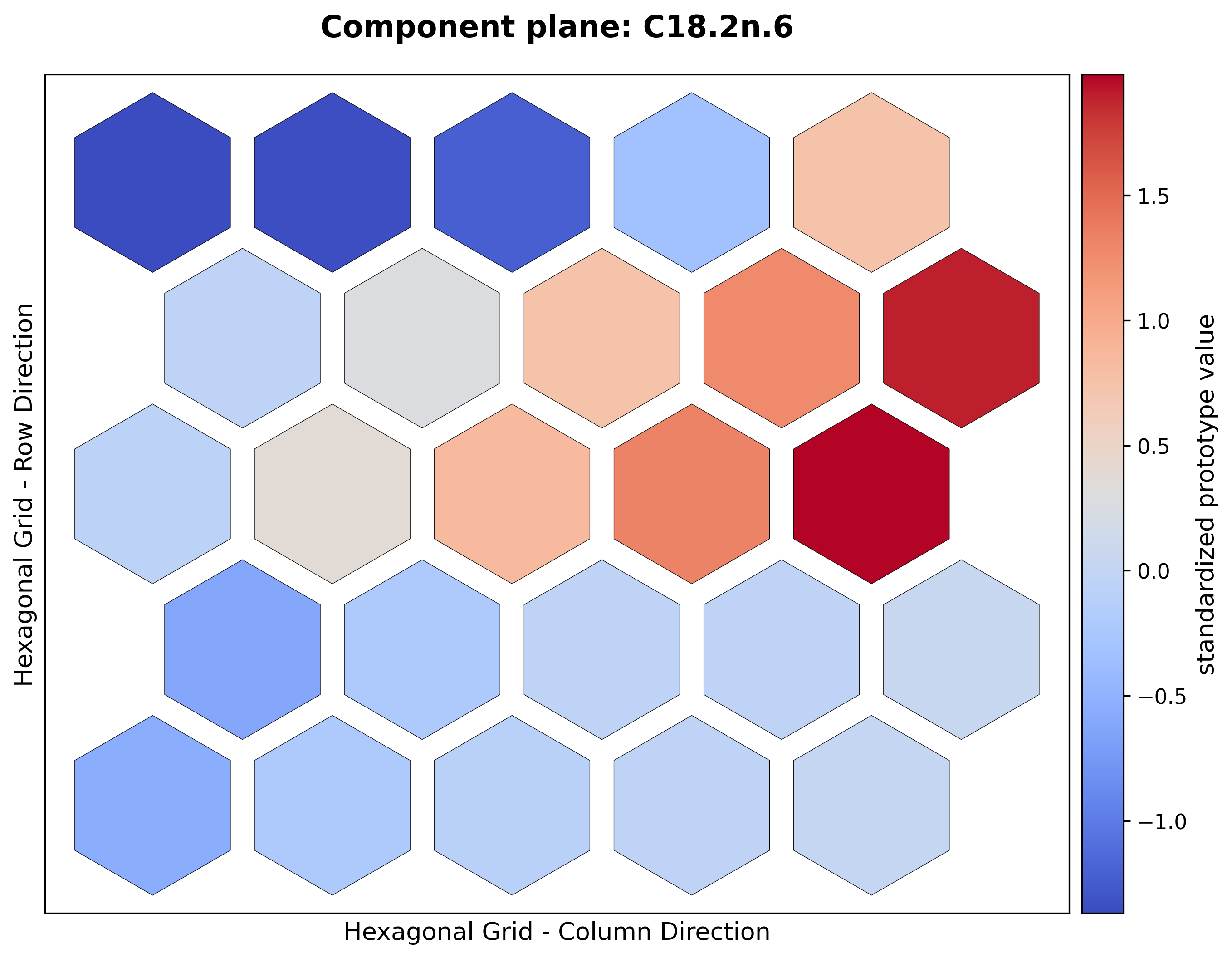
Figure 3.11: Python component plane for C18.2n.6.

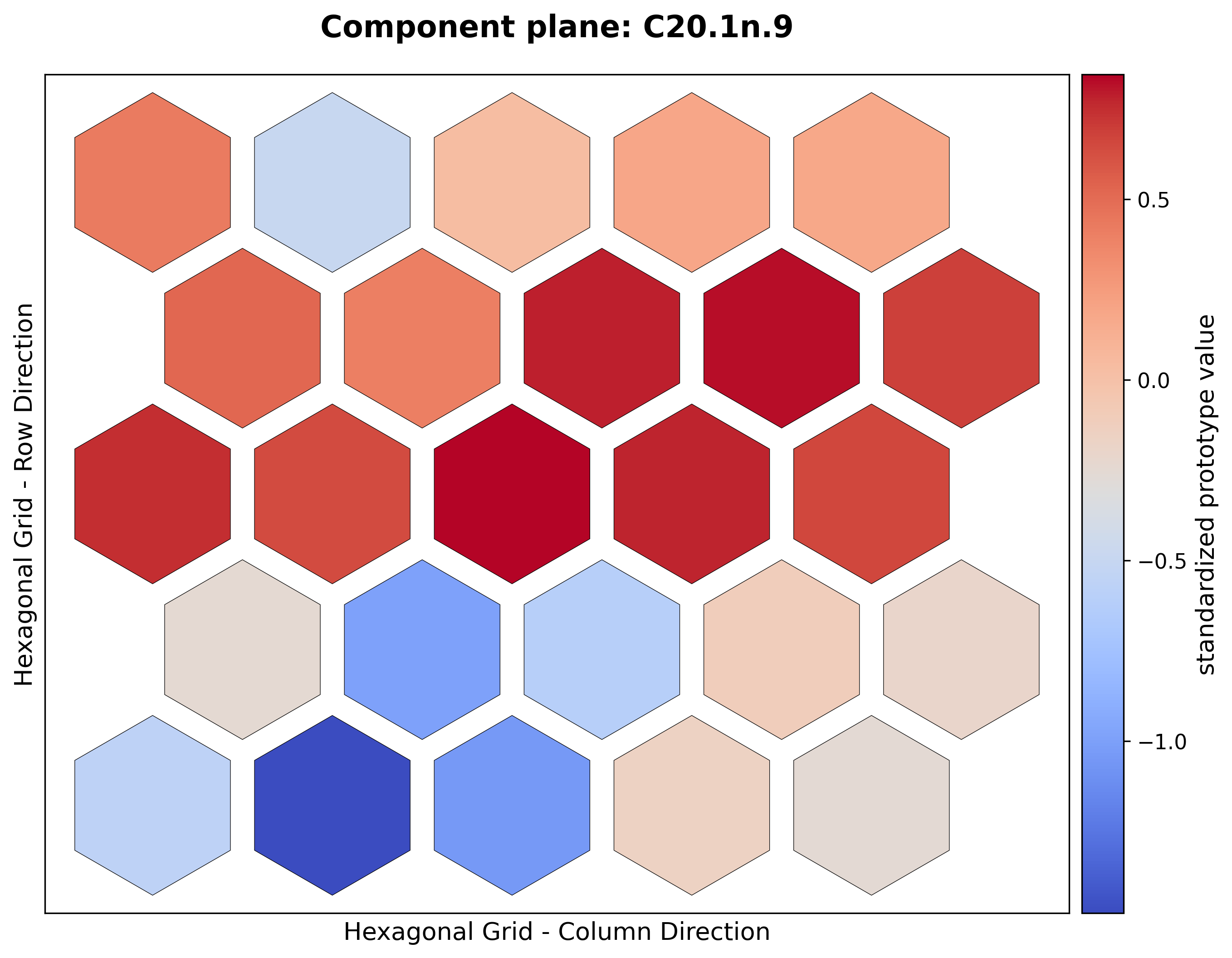
Figure 3.12: Python component plane for C20.1n.9.

C18.2n.6 has a clear gradient across the map. C20.1n.9 has a different pattern. Standardization allowed the lower-variance feature to contribute to distance, but it did not force the two features to tell the same biological story.