2  Diffusion maps in R and Python

The examples use destiny in R and Scanpy in Python with the same observations, features, and neighbor count. The packages construct their graphs differently, so their numerical results differ slightly.

2.1 Simulated data

The dataset contains 900 simulated observations. Progression runs from 0 to 1 and divides into two branches after its midpoint. The data have 30 variables related to this structure and 10 unrelated noise variables.

Four additional columns record the known simulation variables:

• true_pseudotime
• true_branch
• true_latent_x
• true_latent_y

These columns are used to assess the results. They are not included when fitting the diffusion map.

NoteDownload the data

Simulated dataset

R

df <- read.csv(
  "data/diffusion_maps_simulation.csv",
  stringsAsFactors = FALSE
)

feature_cols <- c(
  grep("^x", colnames(df), value = TRUE),
  grep("^nuisance", colnames(df), value = TRUE)
)

dim(df)
length(feature_cols)

[1] 900  45
[1] 40

Python

import numpy as np
import pandas as pd

df = pd.read_csv("data/diffusion_maps_simulation.csv")

feature_cols = [
    c for c in df.columns
    if c.startswith("x") or c.startswith("nuisance")
]

df.shape
len(feature_cols)

(900, 45)
40

Each feature is standardized before the graph is constructed.

R

X <- scale(as.matrix(df[, feature_cols]))

Python

from sklearn.preprocessing import StandardScaler

X = StandardScaler().fit_transform(df[feature_cols].to_numpy())

2.2 PCA comparison

A PCA fit provides a linear comparison.

R

pca <- prcomp(X, center = FALSE, scale. = FALSE)
summary(pca)$importance[2, 1:2]
cor(pca$x[, 1], df$true_pseudotime)
cor(pca$x[, 2], df$true_pseudotime)

   PC1    PC2
0.2130 0.1380
[1] 0.431
[1] -0.369

Python

from sklearn.decomposition import PCA

pca = PCA(n_components=2).fit(X)
pcs = pca.transform(X)

pca.explained_variance_ratio_
np.corrcoef(pcs[:, 0], df["true_pseudotime"])[0, 1]
np.corrcoef(pcs[:, 1], df["true_pseudotime"])[0, 1]

array([0.213, 0.138])
-0.431
-0.369

The sign of a component is arbitrary, so the correlations are compared by magnitude. PC1 and PC2 together account for about 35% of the variance. Neither component follows progression closely.

Figure 2.1: PC1 against PC2, colored by known progression and branch membership.

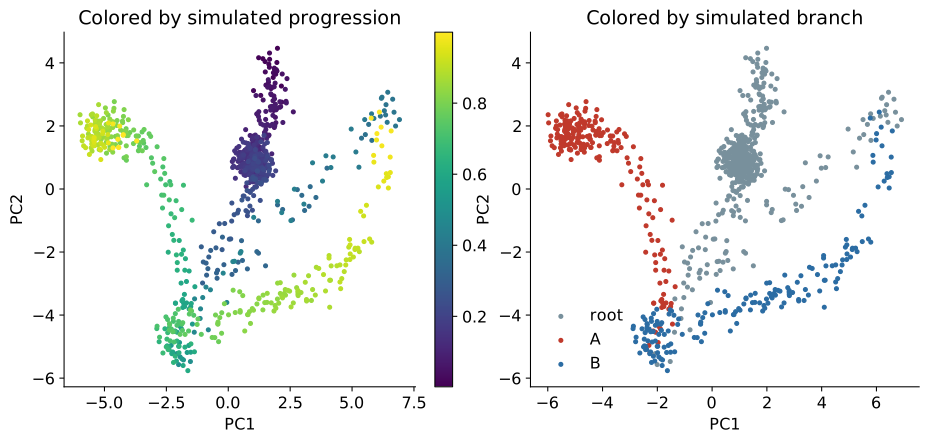
The fork is partly visible, but progression is not represented by a clear PCA axis. A diffusion map instead uses the neighborhood graph.

2.3 Fit a diffusion map

The corresponding settings have different names in the two packages.

Purpose	destiny	Scanpy
Number of neighbors	k	n_neighbors
Kernel	sigma	method in sc.pp.neighbors()
Number of returned components	n_eigs	n_comps
Diffusion coordinates	eigenvectors(dm)	adata.obsm["X_diffmap"]
Eigenvalues	eigenvalues(dm)	adata.uns["diffmap_evals"]

destiny constructs the graph and computes the diffusion map in one call. Scanpy constructs the neighbor graph first and then computes the diffusion map.

R

library(destiny)

set.seed(1)
dm <- DiffusionMap(X, k = 15, n_eigs = 10)

round(eigenvalues(dm)[1:8], 4)

   DC1    DC2    DC3    DC4    DC5    DC6    DC7    DC8
0.9982 0.9956 0.9811 0.9759 0.9596 0.9469 0.9428 0.9242

Python

import anndata as ad
import scanpy as sc

adata = ad.AnnData(X=X.astype("float32"))
sc.pp.neighbors(adata, n_neighbors=15, use_rep="X")
sc.tl.diffmap(adata, n_comps=10)

adata.uns["diffmap_evals"][:8].round(4)

array([1.    , 0.9984, 0.9963, 0.984 , 0.9799, 0.9664, 0.9569, 0.9547])

There is one indexing difference. Scanpy stores the stationary component in column 0. It has eigenvalue 1 and does not separate observations. Scanpy’s DC1 is therefore column 1. destiny omits this component from eigenvectors(dm), so its DC1 is column 1 in R indexing.

Both packages return eigenvectors and eigenvalues separately. The eigenvector columns are the component patterns described in Chapter 1. These outputs can also be combined to form coordinates at a chosen diffusion time.

2.4 Inspect the first components

The first two components can be compared with the known progression variable.

R

dc_r <- eigenvectors(dm)

cor(dc_r[, 1], df$true_pseudotime)
cor(dc_r[, 2], df$true_pseudotime)

[1] 0.9318
[1] -0.2659

Python

dc1_py <- adata.obsm["X_diffmap"][:, 1]
dc2_py <- adata.obsm["X_diffmap"][:, 2]

np.corrcoef(dc1_py, df["true_pseudotime"])[0, 1]
np.corrcoef(dc2_py, df["true_pseudotime"])[0, 1]

-0.9260
-0.2989

DC1 follows progression in both results. Its sign differs because an eigenvector can be multiplied by negative one without changing the geometry. The absolute correlation between the two DC1 vectors is 0.998.

NoteComponent signs

Compare component signs only after aligning their orientation. An opposite sign does not indicate a different embedding.

Figure 2.2: DC1 and DC2 plotted against known progression.

Figure 2.3: DC1 against DC2, colored by known progression and branch membership.

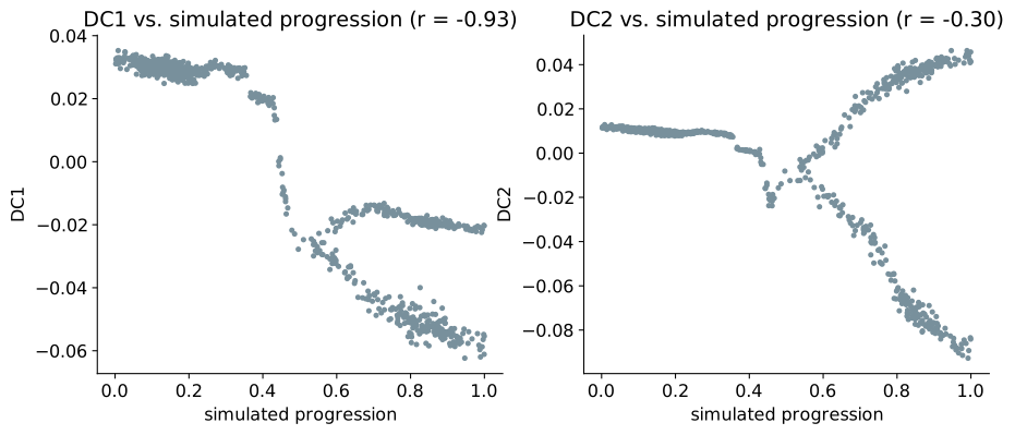
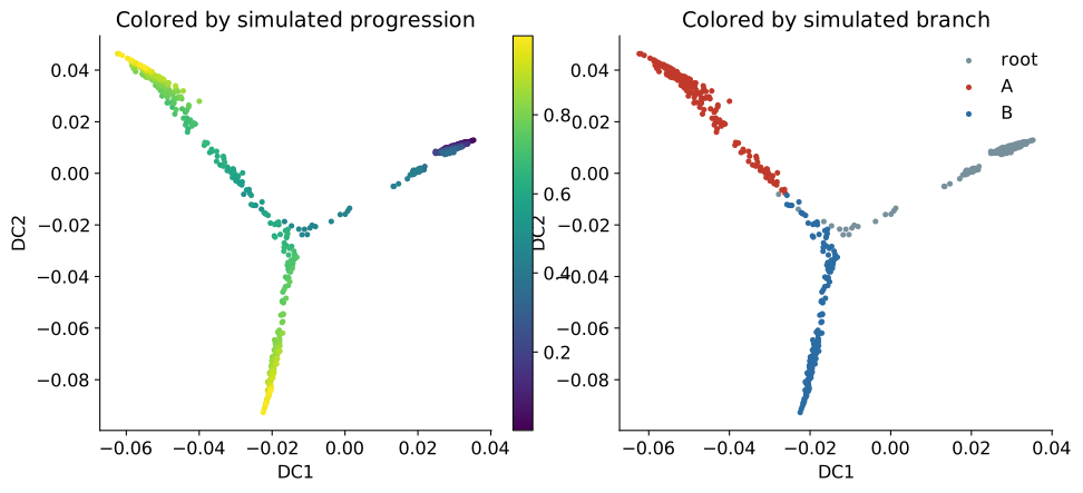
DC1 follows progression and DC2 separates the branches in this simulation. This ordering is specific to this graph. A different dataset can place branch structure or another persistent pattern first.

2.5 Using a fixed diffusion time

destiny and Scanpy return eigenvectors and eigenvalues without requiring a fixed diffusion time. They can be used to construct coordinates at any \(t\):

\[\mathrm{DC}_k^{(t)} = \lambda_k^t\psi_k.\]

Diffusion time explains \(P^t\), diffusion distance, the persistence of graph patterns, and the faster decay of components with smaller eigenvalues. It does not need to be tuned in every analysis.

A fixed \(t>1\) is most relevant when the analysis needs diffusion geometry at a particular propagation scale. Changing \(t\) changes Euclidean distances in the weighted coordinates because each component receives a different weight. Those distances may then be used for clustering, neighbor calculations, or another geometric analysis.

The example below uses \(t=1\), \(t=5\), and \(t=20\). It reports the ranges of DC1 and DC2 and the distance between an early observation and a terminal observation. The distance uses the first nine nonstationary components.

R

evals_r <- eigenvalues(dm)
psi_r <- dc_r[, 1:9]
pair_r <- c(
  which.min(df$true_pseudotime),
  which.max(df$true_pseudotime)
)

for (t in c(1, 5, 20)) {
  coords_t <- sweep(
    psi_r,
    2,
    evals_r[1:9]^t,
    "*"
  )
  span <- apply(coords_t[, 1:2], 2, function(v) diff(range(v)))
  pair_distance <- sqrt(sum(
    (coords_t[pair_r[1], ] - coords_t[pair_r[2], ])^2
  ))
  cat(sprintf(
    "t=%2d  DC1 range=%.4f  DC2 range=%.4f  pair distance=%.4f\n",
    t, span[1], span[2], pair_distance
  ))
}

t= 1  DC1 range=0.0936  DC2 range=0.1395  pair distance=0.1926
t= 5  DC1 range=0.0929  DC2 range=0.1371  pair distance=0.1563
t=20  DC1 range=0.0905  DC2 range=0.1282  pair distance=0.1013

Python

evals_py = adata.uns["diffmap_evals"]
psi_py = adata.obsm["X_diffmap"][:, 1:10]
pair_py = [
    int(df["true_pseudotime"].idxmin()),
    int(df["true_pseudotime"].idxmax()),
]

for t in (1, 5, 20):
    coords_t = psi_py * (evals_py[1:10] ** t)[None, :]
    span = coords_t[:, :2].max(axis=0) - coords_t[:, :2].min(axis=0)
    pair_distance = np.linalg.norm(
        coords_t[pair_py[0]] - coords_t[pair_py[1]]
    )
    print(
        f"t={t:2d}  DC1 range={span[0]:.4f}  "
        f"DC2 range={span[1]:.4f}  "
        f"pair distance={pair_distance:.4f}"
    )

t= 1  DC1 range=0.0975  DC2 range=0.1385  pair distance=0.1972
t= 5  DC1 range=0.0968  DC2 range=0.1365  pair distance=0.1671
t=20  DC1 range=0.0945  DC2 range=0.1290  pair distance=0.1122

The first two eigenvalues are close to 1, so the ranges of DC1 and DC2 change moderately. The pairwise distance changes more because it includes later components with smaller eigenvalues. Those components lose weight faster as \(t\) increases.

Figure 2.4: The first two weighted diffusion coordinates at three values of diffusion time, shown with fixed axis limits.

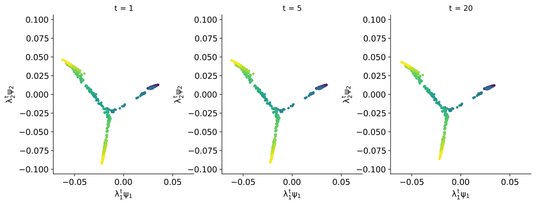
Fixed axis limits are necessary for this comparison. If each panel rescales its axes independently, the plots can look unchanged even when the pairwise distances have decreased.

Many workflows use the returned eigenvectors and eigenvalues directly or use methods such as Diffusion Pseudotime that combine diffusion information across scales. They do not require the analyst to select one fixed \(t\). Very large values are not better because every nonstationary component eventually decays on a connected graph that mixes.

Diffusion time is essential for understanding the method, but choosing a fixed \(t>1\) is not a mandatory step in every practical diffusion map workflow.

2.6 Graph settings

2.6.1 Number of neighbors

The neighbor count controls how many local connections are available to each observation.

R

for (k_try in c(4, 15, 120)) {
  set.seed(1)
  dm_k <- DiffusionMap(X, k = k_try, n_eigs = 5)
  c1 <- cor(eigenvectors(dm_k)[, 1], df$true_pseudotime)
  cat(sprintf(
    "k=%4d  |corr|=%.3f  eigenvalues=%.4f, %.4f\n",
    k_try,
    abs(c1),
    eigenvalues(dm_k)[1],
    eigenvalues(dm_k)[2]
  ))
}

k=   4  |corr|=0.943  eigenvalues=0.9997, 0.9982
k=  15  |corr|=0.932  eigenvalues=0.9982, 0.9956
k= 120  |corr|=0.665  eigenvalues=0.9853, 0.9715

Python

for k_try in (4, 15, 120):
    a = ad.AnnData(X=X.astype("float32"))
    sc.pp.neighbors(a, n_neighbors=k_try, use_rep="X")
    sc.tl.diffmap(a, n_comps=5)
    c1 = np.corrcoef(
        a.obsm["X_diffmap"][:, 1],
        df["true_pseudotime"]
    )[0, 1]
    print(
        f"n_neighbors={k_try:4d}  |corr|={abs(c1):.3f}  "
        f"eigenvalues={a.uns['diffmap_evals'][:2].round(4)}"
    )

n_neighbors=   4  |corr|=0.647  eigenvalues=[1. 1.]
n_neighbors=  15  |corr|=0.926  eigenvalues=[1.     0.9984]
n_neighbors= 120  |corr|=0.683  eigenvalues=[1.     0.9907]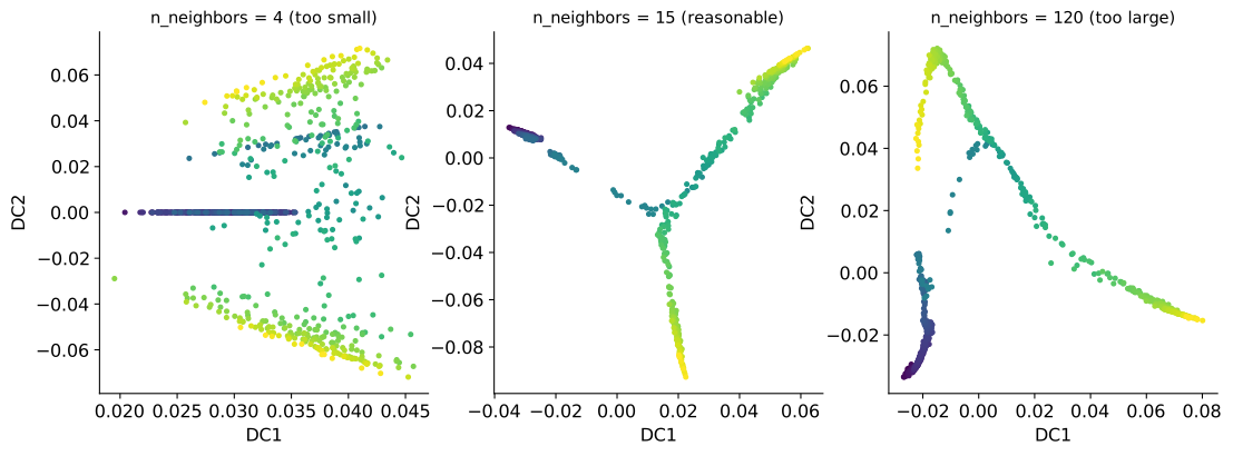

Figure 2.5: Diffusion embeddings with 4, 15, and 120 neighbors.

With 4 neighbors, Scanpy produces a fragmented embedding and destiny remains connected enough to retain the main progression. With 120 neighbors, both methods connect observations across wider regions and the correlation with progression decreases. The same neighbor count does not produce an identical graph in the two packages.

2.6.2 Kernel settings

The packages expose different kernel controls. In destiny, sigma controls the bandwidth. In Scanpy, method selects the connectivity construction. These settings are related but are not direct equivalents.

R

sig <- find_sigmas(X, verbose = FALSE)
sigma_auto <- optimal_sigma(sig)

for (sigma_try in c(1, sigma_auto, 100)) {
  set.seed(1)
  dm_s <- DiffusionMap(
    X,
    k = 15,
    sigma = sigma_try,
    n_eigs = 5
  )
  c1 <- cor(eigenvectors(dm_s)[, 1], df$true_pseudotime)
  cat(sprintf(
    "sigma=%7.3f  |corr|=%.3f\n",
    sigma_try,
    abs(c1)
  ))
}

sigma=  1.000  |corr|=0.797
sigma=  2.934  |corr|=0.928
sigma=100.000  |corr|=0.919

Python

for method in ("umap", "gauss"):
    a = ad.AnnData(X=X.astype("float32"))
    sc.pp.neighbors(
        a,
        n_neighbors=15,
        method=method,
        use_rep="X"
    )
    sc.tl.diffmap(a, n_comps=5)
    c1 = np.corrcoef(
        a.obsm["X_diffmap"][:, 1],
        df["true_pseudotime"]
    )[0, 1]
    print(f"method={method:6s}  |corr|={abs(c1):.3f}")

method=umap    |corr|=0.926
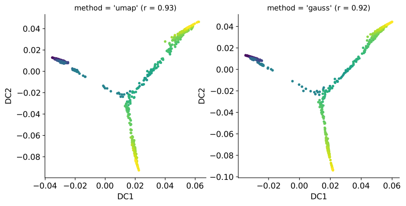
method=gauss   |corr|=0.919

A narrow bandwidth in destiny weakens communication beyond the closest observations and reduces the progression correlation. The broad bandwidth has a smaller effect because the neighbor count still limits which pairs can be connected. Scanpy’s two kernel methods give similar results on this dataset.

Figure 2.6: Scanpy diffusion embeddings using the UMAP and Gaussian connectivity methods.

destiny also provides density_norm. Scanpy does not expose an equivalent switch, so the settings are not directly comparable. Density normalization is derived in Chapter 3.

2.6.3 Number of components

Both packages return more components when requested. The first nine are compared with known progression and with one of the simulated noise variables.

R

for (i in 1:9) {
  c_progress <- cor(dc_r[, i], df$true_pseudotime)
  c_noise <- cor(dc_r[, i], df$nuisance_01)
  cat(sprintf(
    "DC%d  progression=%+.3f  nuisance=%+.3f\n",
    i, c_progress, c_noise
  ))
}

DC1  progression=+0.932  nuisance=-0.044
DC2  progression=-0.266  nuisance=-0.006
DC3  progression=-0.122  nuisance=-0.018
DC4  progression=+0.173  nuisance=-0.068
DC5  progression=+0.028  nuisance=+0.079
DC6  progression=-0.059  nuisance=+0.100
DC7  progression=+0.048  nuisance=+0.000
DC8  progression=-0.035  nuisance=+0.012
DC9  progression=+0.002  nuisance=+0.004

Python

components_py = adata.obsm["X_diffmap"][:, 1:10]

for i in range(9):
    c_progress = np.corrcoef(
        components_py[:, i],
        df["true_pseudotime"]
    )[0, 1]
    c_noise = np.corrcoef(
        components_py[:, i],
        df["nuisance_01"]
    )[0, 1]
    print(
        f"DC{i + 1}  progression={c_progress:+.3f}  "
        f"nuisance={c_noise:+.3f}"
    )

DC1  progression=-0.926  nuisance=+0.047
DC2  progression=-0.299  nuisance=-0.003
DC3  progression=-0.120  nuisance=-0.015
DC4  progression=-0.155  nuisance=+0.074
DC5  progression=-0.036  nuisance=-0.074
DC6  progression=-0.058  nuisance=+0.106
DC7  progression=+0.040  nuisance=+0.012
DC8  progression=+0.038  nuisance=-0.021
DC9  progression=-0.001  nuisance=-0.002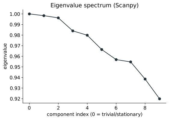

Figure 2.7: Scanpy eigenvalues, including the stationary component at index 0.

The spectrum has no clear cutoff. DC1 has the strongest relationship with progression. Later components have weaker relationships with progression and may describe branch structure or finer variation. None of these nine components correlates strongly with the selected noise variable. This check does not prove that every later component is useful or that all technical effects have been removed.

The number of retained components should be chosen from the downstream task, the eigenvalue pattern, and the stability and interpretation of the component values.

2.7 Diffusion pseudotime

Diffusion coordinates describe geometry without assigning a direction. Diffusion Pseudotime uses a selected root observation to orient that geometry.

The root below is the observation with the smallest known simulation time. With observed data, the root must be supported by experimental information or subject knowledge.

R

root_r <- which.min(df$true_pseudotime)
dpt_r <- DPT(dm, tips = root_r)

round(cor(dpt_r$DPT1, df$true_pseudotime), 3)

[1] 0.96

Python

root_py = int(df["true_pseudotime"].idxmin())
adata.uns["iroot"] = root_py
sc.tl.dpt(adata, n_branchings=0)

round(np.corrcoef(
    adata.obs["dpt_pseudotime"],
    df["true_pseudotime"]
)[0, 1], 3)

0.962

Both implementations recover an ordering close to the known progression. This result depends on the selected root. Neither diffusion maps nor Diffusion Pseudotime can identify the biological starting state without additional information.