4 NMF on leukemia gene expression data
These exercises apply non-negative matrix factorization (NMF) to the acute leukemia gene expression dataset studied by Golub et al. (1999) and Brunet et al. (2004). The dataset contains 38 bone-marrow samples and measurements for 5,000 genes. Each sample is labelled as acute lymphoblastic leukemia (ALL) or acute myeloid leukemia (AML). The ALL samples are further divided into B-cell and T-cell subtypes.
The labels will not be supplied to NMF. They will be used only after fitting to help interpret the components.
Choose either R or Python and use that language throughout the chapter. Run only the code in your chosen tab.
The exercises form one sequential analysis. Keep the same session open as you work. Every exercise begins by listing the objects it requires and ends with a checkpoint listing the objects needed later.
4.1 NMF notation used in the exercises
The expression matrix is arranged with samples in rows and genes in columns:
\[ X \in \mathbb{R}_{\geq 0}^{38 \times 5000}. \]
At rank \(k\), NMF approximates this matrix as
\[ X \approx WH, \]
where
\[ W \in \mathbb{R}_{\geq 0}^{38 \times k} \qquad\text{and}\qquad H \in \mathbb{R}_{\geq 0}^{k \times 5000}. \]
- A row of \(W\) contains the component scores for one sample.
- A row of \(H\) contains the gene profile for one component.
- The product \(WH\) is the reconstructed expression matrix.
Place the three files inside a folder named data in your working directory.
4.2 Exercise 1. Load and check the data
Starting objects: none
Goal: Create the data objects used throughout the chapter and verify that the matrix is suitable for NMF.
Task.
- Load the expression matrix and sample metadata.
- Store the numerical expression matrix as
X. - Store the 5,000 probe identifiers as
gene_names. - Create a three-class sample label called
group, with valuesALL-B-cell,ALL-T-cell, andAML. - Confirm that
Xhas 38 sample rows and 5,000 gene columns, contains no negative values, and contains no missing values. - Report the number of samples in each group.
The first column of the expression file contains sample identifiers. It should become the row names in R or the index in Python, not a numerical column of X.
expr <- read.csv("data/golub_expression.csv", row.names = 1)
meta <- read.csv("data/golub_metadata.csv")

X <- as.matrix(expr)
gene_names <- colnames(X)

group <- ifelse(
  meta$ALL_AML == "AML",
  "AML",
  paste0("ALL-", meta$cell_type)
)

stopifnot(identical(rownames(expr), meta$sample_id))

dim(X)
range(X)
any(X < 0)
any(is.na(X))
table(group)
import numpy as np
import pandas as pd
expr = pd.read_csv("data/golub_expression.csv", index_col=0)
meta = pd.read_csv("data/golub_metadata.csv")
X = expr.to_numpy()
gene_names = expr.columns.to_numpy()
group = np.where(
meta["ALL_AML"].eq("AML"),
"AML",
"ALL-" + meta["cell_type"].astype(str),
)
assert np.array_equal(expr.index.to_numpy(), meta["sample_id"].to_numpy())
print(X.shape)
print(X.min(), X.max())
print((X < 0).any())
print(pd.isna(X).any())
print(pd.Series(group).value_counts())The checks should report a \(38 \times 5000\) matrix, a range from 20 to 61,225, no negative values, and no missing values. The three groups contain 19 B-cell ALL samples, 8 T-cell ALL samples, and 11 AML samples.
Keep these four objects:
X: \(38 \times 5000\)expr: 38 samples by 5,000 genes, including namesgene_names: length 5,000group: length 38
4.3 Exercise 2. Examine reconstruction error across ranks
Starting object: X
Goal: Determine what training reconstruction error can and cannot tell us about the NMF rank.
For a fitted reconstruction \(\widehat X=WH\), the root mean squared reconstruction error is
\[ \operatorname{RMSE} = \sqrt{\frac{1}{np}\sum_{i=1}^{n}\sum_{j=1}^{p} (X_{ij}-\widehat X_{ij})^2}. \]
Task.
- Fit NMF at ranks 2 through 8 using the full 5,000-gene matrix.
- Store the RMSE at each rank in
rank_rmse. - Plot RMSE against rank.
- Decide whether the rank with the lowest training RMSE must be the most useful rank.
library(NNLM)

candidate_ranks <- 2:8
rank_rmse <- numeric(length(candidate_ranks))

for (i in seq_along(candidate_ranks)) {
  k <- candidate_ranks[i]
  set.seed(100 + k)
  rank_fit <- nnmf(
    X,
    k = k,
    method = "scd",
    loss = "mse",
    max.iter = 1000,
    rel.tol = 1e-4,
    verbose = 0
  )
  X_rank_hat <- rank_fit$W %*% rank_fit$H
  rank_rmse[i] <- sqrt(mean((X - X_rank_hat)^2))
}

names(rank_rmse) <- candidate_ranks
round(rank_rmse, 1)

plot(
  candidate_ranks,
  rank_rmse,
  type = "b",
  xlab = "Rank k",
  ylab = "Training RMSE"
)
import matplotlib.pyplot as plt
from sklearn.decomposition import NMF
candidate_ranks = range(2, 9)
rank_rmse = {}
for k in candidate_ranks:
rank_model = NMF(
n_components=k,
init="nndsvda",
solver="cd",
beta_loss="frobenius",
max_iter=1000,
tol=1e-4,
random_state=0,
)
W_rank = rank_model.fit_transform(X)
X_rank_hat = W_rank @ rank_model.components_
rank_rmse[k] = np.sqrt(np.mean((X - X_rank_hat) ** 2))
print({k: round(value, 1) for k, value in rank_rmse.items()})
plt.plot(list(rank_rmse), list(rank_rmse.values()), marker="o")
plt.xlabel("Rank k")
plt.ylabel("Training RMSE")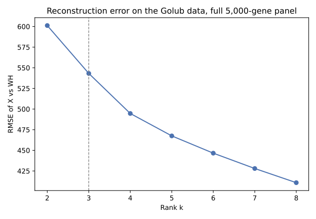
The observed RMSE decreases smoothly from about 601 at rank 2 to about 410 at rank 8. The best achievable training error cannot increase when extra components are available, although an individual non-convex optimization run can occasionally return a poorer local solution. Consequently, the lowest training error in this sweep is not sufficient evidence that rank 8 is the most stable or interpretable choice.
No objects from this exercise are required later.
4.4 Exercise 3. Choose a rank using consensus stability
Starting objects: X, group
Goal: Evaluate whether sample assignments are reproducible across repeated NMF fits.
Running NMF from different random initializations can produce different sample assignments. For one rank, define a connectivity matrix for each run:
\[ C_{ij}^{(b)}= \begin{cases} 1, & \text{if samples }i\text{ and }j\text{ have the same dominant component},\\ 0, & \text{otherwise.} \end{cases} \]
The consensus matrix is the average of these connectivity matrices across runs. Its entries lie between 0 and 1. Values near 1 mean that a pair of samples is repeatedly assigned together. Values near 0 mean that the pair is repeatedly separated. A clear block pattern indicates stable assignments. Cophenetic correlation summarizes how clearly the consensus matrix supports a hierarchical grouping. Values closer to 1 indicate a clearer structure.
Repeated fits are slower than a single fit. For this exercise only, use the 1,000 genes with the largest variance across samples. The filter must be calculated without using group.
Task.
- Select the 1,000 most variable genes and store the reduced matrix as
X_filtered. - For ranks 2 through 6, run 15 NMF fits with different random initializations.
- Store the cophenetic correlations as
cophenetic_by_rank. - Store the rank-2 and rank-3 consensus matrices as
consensus_k2andconsensus_k3. - Compare the correlations and consensus matrices, then store the selected rank as
chosen_rank.
The known leukemia labels are not used to select genes, fit NMF, construct the consensus matrices, or calculate cophenetic correlation. They are used only afterward to arrange the heatmaps so that their biological meaning is easier to inspect.
The NMF package performs the repeated fits and constructs the consensus matrices. For this package, samples must be in columns when sample consensus is calculated, so X_filtered is transposed in the call to nmf().
library(NMF)

gene_variance <- apply(X, 2, var)
selected_genes <- order(gene_variance, decreasing = TRUE)[1:1000]
X_filtered <- X[, selected_genes]

survey <- nmf(
  t(X_filtered),
  rank = 2:6,
  nrun = 15,
  method = "brunet",
  seed = 123
)

cophenetic_by_rank <- sapply(survey$fit, cophcor)
names(cophenetic_by_rank) <- 2:6

consensus_k2 <- consensus(survey$fit[["2"]])
consensus_k3 <- consensus(survey$fit[["3"]])

round(cophenetic_by_rank, 4)
2 3 4 5 6
0.9908 1.0000 0.9686 0.9833 0.9790sample_order <- order(group)
old_par <- par(mfrow = c(1, 2), mar = c(3, 3, 3, 1))
image(
consensus_k2[sample_order, sample_order],
axes = FALSE,
main = "Consensus, k = 2",
col = hcl.colors(50, "YlOrRd", rev = TRUE)
)
image(
consensus_k3[sample_order, sample_order],
axes = FALSE,
main = "Consensus, k = 3",
col = hcl.colors(50, "YlOrRd", rev = TRUE)
)
par(old_par)
chosen_rank <- 3Lscikit-learn fits NMF but does not construct a consensus survey automatically. The supplied function below performs the repeated fits and returns the consensus matrix and cophenetic correlation for every candidate rank.
from scipy.cluster.hierarchy import cophenet, linkage
from scipy.spatial.distance import squareform
from sklearn.decomposition import NMF


def nmf_consensus_survey(X, ranks, n_runs=15, seed=123):
    """Calculate NMF consensus matrices and cophenetic correlations.

    X must have samples in rows and features in columns.
    The returned dictionary is indexed by rank.
    """
    results = {}
    n_samples = X.shape[0]

    for k in ranks:
        # Count how often every pair of samples is assigned together.
        same_component = np.zeros((n_samples, n_samples))

        for run in range(n_runs):
            model = NMF(
                n_components=k,
                init="random",
                solver="mu",
                beta_loss="kullback-leibler",
                max_iter=500,
                tol=1e-4,
                random_state=seed + run,
            )
            W_run = model.fit_transform(X)
            labels = W_run.argmax(axis=1)
            same_component += labels[:, None] == labels[None, :]

        # Convert the counts to proportions between 0 and 1.
        consensus = same_component / n_runs

        # Convert consensus similarity to a distance and summarize it.
        distance = squareform(1 - consensus, checks=False)
        tree = linkage(distance, method="average")
        cophenetic = cophenet(tree, distance)[0]

        results[k] = {
            "consensus": consensus,
            "cophenetic": cophenetic,
        }

    return results
gene_variance = X.var(axis=0)
selected_genes = np.argsort(gene_variance)[::-1][:1000]
X_filtered = X[:, selected_genes]
survey = nmf_consensus_survey(
X_filtered,
ranks=range(2, 7),
n_runs=15,
seed=123,
)
cophenetic_by_rank = pd.Series({
k: survey[k]["cophenetic"] for k in survey
})
consensus_k2 = survey[2]["consensus"]
consensus_k3 = survey[3]["consensus"]
print(cophenetic_by_rank.round(4))2 0.9923
3 0.9965
4 0.9553
5 0.9359
6 0.9544sample_order = np.argsort(group)
fig, axes = plt.subplots(1, 2, figsize=(10, 4.5))
axes[0].imshow(
consensus_k2[np.ix_(sample_order, sample_order)],
vmin=0,
vmax=1,
cmap="YlOrRd",
)
axes[0].set_title("Consensus, k = 2")
axes[1].imshow(
consensus_k3[np.ix_(sample_order, sample_order)],
vmin=0,
vmax=1,
cmap="YlOrRd",
)
axes[1].set_title("Consensus, k = 3")
for ax in axes:
ax.set_xlabel("Samples")
ax.set_ylabel("Samples")
chosen_rank = 3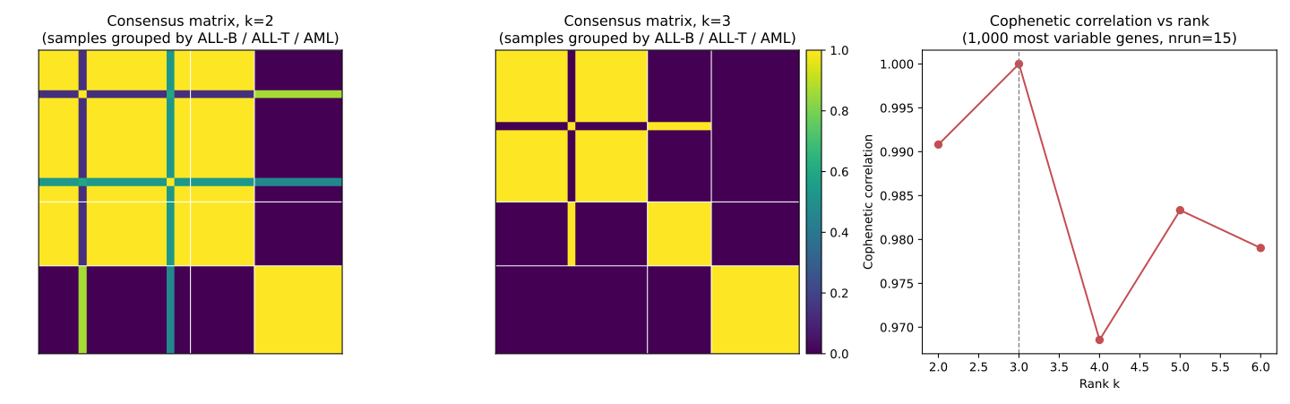
The survey identifies rank 3 as the strongest candidate. At rank 2, the two ALL subtypes are usually placed together. At rank 3, B-cell ALL, T-cell ALL, and AML form three much clearer blocks. Exact correlation values can vary with the NMF algorithm, but the rank should be selected from the stability pattern rather than by requiring one particular decimal value.
Keep chosen_rank, which should equal 3. The other objects from this exercise are not required for the final fit.
4.5 Exercise 4. Fit the final model and fix its scale
Starting objects: X, chosen_rank
Goal: Fit the rank-3 model once and put its components on a defined, comparable scale.
NMF has a scaling ambiguity. For any positive diagonal matrix \(D\),
\[ WH=(WD)(D^{-1}H). \]
Consequently, raw columns of \(W\) need not be directly comparable. We will impose one convention: every row of \(H\) will sum to 1. Define
\[ s_r=\sum_j H_{rj}, \qquad H^{*}_{rj}=\frac{H_{rj}}{s_r}, \qquad W^{*}_{ir}=W_{ir}s_r. \]
This changes the factor scales but leaves the reconstruction unchanged:
\[ W^{*}H^{*}=WH. \]
Task.
- Fit NMF at
chosen_rankusing the full 5,000-gene matrix. - Store the direct model output as
W_rawandH_raw. - Store the row sums of
H_rawascomponent_scale. - Create
W_scaledandH_profileusing the equations above. - Confirm that every row of
H_profilesums to 1 and that the reconstruction has not changed.
library(NNLM)

set.seed(1)
model3 <- nnmf(
  X,
  k = chosen_rank,
  method = "scd",
  loss = "mse",
  max.iter = 2000,
  rel.tol = 1e-8,
  verbose = 0
)

W_raw <- model3$W
H_raw <- model3$H

component_scale <- rowSums(H_raw)
stopifnot(all(component_scale > 0))

W_scaled <- sweep(W_raw, 2, component_scale, "*")
H_profile <- sweep(H_raw, 1, component_scale, "/")

dim(W_scaled)
dim(H_profile)
rowSums(H_profile)
max(abs(W_raw %*% H_raw - W_scaled %*% H_profile))
from sklearn.decomposition import NMF
model3 = NMF(
n_components=chosen_rank,
init="nndsvda",
solver="cd",
beta_loss="frobenius",
max_iter=2000,
tol=1e-6,
random_state=0,
)
W_raw = model3.fit_transform(X)
H_raw = model3.components_
component_scale = H_raw.sum(axis=1)
if np.any(component_scale <= 0):
raise ValueError("The fit contains an empty component")
W_scaled = W_raw * component_scale[None, :]
H_profile = H_raw / component_scale[:, None]
print(W_scaled.shape)
print(H_profile.shape)
print(H_profile.sum(axis=1))
print(np.max(np.abs(W_raw @ H_raw - W_scaled @ H_profile)))W_scaled should be \(38 \times 3\), H_profile should be \(3 \times 5000\), and every row of H_profile should sum to 1. Any reported reconstruction difference should be at numerical rounding level.
Keep W_scaled and H_profile. Do not refit the model in later exercises.
4.6 Exercise 5. Interpret the sample scores
Starting objects: expr, group, W_scaled, H_profile
Goal: Identify the dominant fitted component for each sample and give the arbitrary component numbers meaningful names.
Because each row of H_profile sums to 1, the entries in one row of W_scaled can be converted into within-sample fractions:
\[ q_{ir}=\frac{W^{*}_{ir}}{\sum_s W^{*}_{is}}. \]
The largest fraction identifies the dominant component, while the full row shows whether a sample is strongly dominated by one component or contains substantial contributions from several components.
The Adjusted Rand Index (ARI) compares two partitions while accounting for agreement expected by chance. An ARI of 1 indicates identical partitions. A value near 0 indicates little agreement beyond chance.
Task.
- Find each sample’s dominant component.
- Cross-tabulate the dominant components against
groupand calculate the ARI. - Use the cross-tabulation to associate each fitted component with
ALL-B-cell,ALL-T-cell, orAML. - Reorder the factors into that biological order and store them as
W_namedandH_named. - Store the within-sample fractions as
sample_fractions. - Find the sample with the smallest largest fraction and store its identifier as
mixed_sample.
The known labels are used here only to name and evaluate components after fitting. They were not used to choose genes, select the rank, or fit the final model.
library(mclust)

# Component numbers are 1, 2, and 3.
dominant_component <- max.col(W_scaled, ties.method = "first")
component_table <- table(dominant_component, group)
component_table

ari <- adjustedRandIndex(dominant_component, group)
round(ari, 4)

# Give each component the name of the group most often assigned to it.
component_names <- colnames(component_table)[
  max.col(component_table, ties.method = "first")
]
names(component_names) <- rownames(component_table)
component_names

# Reorder the factors so that later code can use biological names.
group_order <- c("ALL-B-cell", "ALL-T-cell", "AML")
component_for_group <- setNames(
  as.integer(names(component_names)),
  component_names
)
component_order <- component_for_group[group_order]

W_named <- W_scaled[, component_order, drop = FALSE]
H_named <- H_profile[component_order, , drop = FALSE]

rownames(W_named) <- rownames(expr)
colnames(W_named) <- group_order
rownames(H_named) <- group_order
colnames(H_named) <- colnames(expr)

sample_fractions <- W_named / rowSums(W_named)
dominant_name <- colnames(W_named)[
  max.col(W_named, ties.method = "first")
]
table(fitted = dominant_name, known = group)

largest_fraction <- apply(sample_fractions, 1, max)
mixed_sample <- names(which.min(largest_fraction))
mixed_sample
round(sample_fractions[mixed_sample, ], 3)
from sklearn.metrics import adjusted_rand_score
# Use the component numbers 1, 2, and 3.
dominant_component = W_scaled.argmax(axis=1) + 1
component_table = pd.crosstab(
pd.Series(dominant_component, name="component"),
pd.Series(group, name="group"),
)
print(component_table)
ari = adjusted_rand_score(group, dominant_component)
print(round(ari, 4))
# Give each component the name of the group most often assigned to it.
component_names = component_table.idxmax(axis=1).to_dict()
print(component_names)
# Reorder the factors so that later code can use biological names.
group_order = ["ALL-B-cell", "ALL-T-cell", "AML"]
component_for_group = {
name: component for component, name in component_names.items()
}
component_order = [component_for_group[name] - 1 for name in group_order]
W_named = pd.DataFrame(
W_scaled[:, component_order],
index=expr.index,
columns=group_order,
)
H_named = pd.DataFrame(
H_profile[component_order, :],
index=group_order,
columns=expr.columns,
)
sample_fractions = W_named.div(W_named.sum(axis=1), axis=0)
dominant_name = W_named.idxmax(axis=1)
print(pd.crosstab(dominant_name, group))
largest_fraction = sample_fractions.max(axis=1)
mixed_sample = largest_fraction.idxmin()
print(mixed_sample)
print(sample_fractions.loc[mixed_sample].round(3))After the L1 scaling convention, the dominant components have an ARI of approximately 0.76 against the three known groups. All B-cell and T-cell ALL samples have the expected dominant component. 8 of the 11 AML samples are AML-dominant, while 3 have a larger B-cell-component score. This is useful agreement, but it is not perfect classification, nor should NMF be treated as a supervised classifier.
sample_37 is the least dominated by a single component. Its approximate fractions are 0.438 B-cell, 0.125 T-cell, and 0.436 AML. It is therefore a useful sample for examining how several component contributions add together.
Keep:
W_named: \(38 \times 3\), with named component columnsH_named: \(3 \times 5000\), with named component rowssample_fractions: \(38 \times 3\)mixed_sample: the identifiersample_37
4.7 Exercise 6. Reconstruct one sample and the full matrix
Starting objects: X, expr, gene_names, W_named, H_named, mixed_sample
Goal: Connect the fitted factors directly to reconstructed gene expression.
For sample \(i\) and gene \(j\),
\[ \widehat X_{ij} = \sum_{r=1}^{3}W^{*}_{ir}H^{*}_{rj}. \]
Each term is the contribution of one component. Adding the three component contributions produces the reconstructed sample.
Task.
- For
mixed_sample, multiply each row ofH_namedby the matching entry in that sample’s row ofW_named. - Store the resulting component-by-gene matrix as
sample_contributions. - Sum its rows to obtain
sample_reconstruction. - Construct the full reconstruction
X_hatand confirm that its row formixed_sampleequalssample_reconstruction. - Store
X - X_hatasresidualand calculate the overall RMSE. - Identify the eight genes with the largest mean absolute residual.
sample_index <- match(mixed_sample, rownames(expr))

sample_contributions <- sweep(
  H_named,
  1,
  W_named[mixed_sample, ],
  "*"
)
sample_reconstruction <- colSums(sample_contributions)

X_hat <- W_named %*% H_named
stopifnot(isTRUE(all.equal(
  as.numeric(sample_reconstruction),
  as.numeric(X_hat[sample_index, ]),
  tolerance = 1e-10
)))

residual <- X - X_hat
overall_rmse <- sqrt(mean(residual^2))
overall_rmse

mean_absolute_residual <- colMeans(abs(residual))
head(sort(mean_absolute_residual, decreasing = TRUE), 8)
sample_index = expr.index.get_loc(mixed_sample)
sample_contributions = H_named.mul(
W_named.loc[mixed_sample],
axis=0,
)
sample_reconstruction = sample_contributions.sum(axis=0)
X_hat = W_named.to_numpy() @ H_named.to_numpy()
assert np.allclose(sample_reconstruction, X_hat[sample_index])
residual = X - X_hat
overall_rmse = np.sqrt(np.mean(residual**2))
print(overall_rmse)
mean_absolute_residual = pd.Series(
np.abs(residual).mean(axis=0),
index=gene_names,
)
print(mean_absolute_residual.nlargest(8))The overall RMSE is approximately 543.2, matching the rank-3 result from Exercise 2. The equality check confirms that reconstructing one sample component by component is exactly the same calculation as taking the corresponding row of the matrix product.
No objects from this exercise are required later.
4.8 Exercise 7. Identify the genes defining each component
Starting object: H_named
Goal: Use the fitted component profiles to identify and annotate the genes with the largest weights.
Within one row of H_named, a larger value means that the gene contributes more strongly to that component profile. Because the rows have been given biological names, results can now be reported by component meaning rather than by arbitrary component number.
Task.
- Load
data/golub_gene_symbols.csvasgene_annotation. - For each row of
H_named, select the eight genes with the largest weights. - Join their probe identifiers to their gene symbols and full names.
- Store the three annotated tables in
top_genes. - Describe whether each component’s high-weight genes form a coherent biological pattern.
gene_annotation <- read.csv("data/golub_gene_symbols.csv")
top_genes <- list()

for (component in rownames(H_named)) {
  weights <- sort(
    H_named[component, ],
    decreasing = TRUE
  )[1:8]

  annotation_row <- match(
    names(weights),
    gene_annotation$feature_id
  )

  top_table <- data.frame(
    feature_id = names(weights),
    symbol = gene_annotation$symbol[annotation_row],
    genename = gene_annotation$genename[annotation_row],
    weight = as.numeric(weights)
  )

  top_genes[[component]] <- top_table
  cat("\n", component, "\n", sep = "")
  print(top_table[, c("feature_id", "symbol", "weight")])
}
gene_annotation = pd.read_csv(
"data/golub_gene_symbols.csv",
index_col="feature_id",
)
top_genes = {}
for component in H_named.index:
weights = H_named.loc[component].nlargest(8)
top_table = weights.rename("weight").to_frame()
top_table = top_table.join(
gene_annotation[["symbol", "genename"]]
)
top_table = top_table[["symbol", "genename", "weight"]]
top_genes[component] = top_table
print(f"\n{component}")
print(top_table[["symbol", "weight"]].round(4))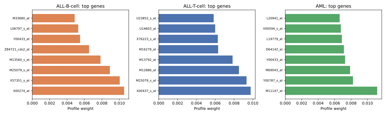
The T-cell component contains T-cell receptor genes together with LCK, CD99, and MAL, giving it a clear lymphoid interpretation. The B-cell component includes the antigen-presentation genes HLA-DRA and CD74, as well as CD81. The AML component contains FTL, FTH1, CXCL8, and NFKBIA, together with genes associated with more general cellular activity. Its profile is less cell-type-specific than the two ALL profiles.
Keep top_genes. It is used to highlight genes in the final loading plot.
4.9 Exercise 8. Connect score and loading plots
Starting objects: W_named, H_named, group, top_genes
Goal: Relate the samples carrying a component to the genes defining that component.
A score plot places samples using columns of W_named. A loading plot places genes using rows of H_named. The axes refer to the same components, but the points represent different objects: samples in the first plot and genes in the second.
Task.
- Make a sample score plot using the AML and B-cell component columns of
W_named. - Colour the samples by
group. - Make a gene loading plot using the AML and B-cell component rows of
H_named. - Highlight the top eight AML genes and top eight B-cell genes stored in
top_genes. - Explain what can be learned from each plot and how the two plots are connected.
group_factor <- factor(
  group,
  levels = c("ALL-B-cell", "ALL-T-cell", "AML")
)
group_colours <- c("steelblue", "darkorange", "firebrick")

plot(
  W_named[, "AML"],
  W_named[, "ALL-B-cell"],
  col = group_colours[group_factor],
  pch = 19,
  xlab = "AML component score",
  ylab = "B-cell component score"
)
legend(
  "topright",
  legend = levels(group_factor),
  col = group_colours,
  pch = 19
)
top_aml_ids <- top_genes[["AML"]]$feature_id
top_bcell_ids <- top_genes[["ALL-B-cell"]]$feature_id
plot(
H_named["AML", ],
H_named["ALL-B-cell", ],
pch = 19,
col = "grey75",
cex = 0.5,
xlab = "AML profile weight",
ylab = "B-cell profile weight"
)
points(
H_named["AML", top_aml_ids],
H_named["ALL-B-cell", top_aml_ids],
col = "firebrick",
pch = 19
)
points(
H_named["AML", top_bcell_ids],
H_named["ALL-B-cell", top_bcell_ids],
col = "steelblue",
pch = 19
)
abline(0, 1, lty = 2)import matplotlib.pyplot as plt
group_colours = {
"ALL-B-cell": "steelblue",
"ALL-T-cell": "darkorange",
"AML": "firebrick",
}
fig, ax = plt.subplots(figsize=(6.5, 5.5))
for label, colour in group_colours.items():
selected = group == label
ax.scatter(
W_named.loc[selected, "AML"],
W_named.loc[selected, "ALL-B-cell"],
label=label,
color=colour,
)
ax.set_xlabel("AML component score")
ax.set_ylabel("B-cell component score")
ax.legend()top_aml_ids = top_genes["AML"].index
top_bcell_ids = top_genes["ALL-B-cell"].index
fig, ax = plt.subplots(figsize=(6.5, 5.5))
ax.scatter(
H_named.loc["AML"],
H_named.loc["ALL-B-cell"],
color="lightgrey",
s=12,
)
ax.scatter(
H_named.loc["AML", top_aml_ids],
H_named.loc["ALL-B-cell", top_aml_ids],
color="firebrick",
label="Top AML genes",
)
ax.scatter(
H_named.loc["AML", top_bcell_ids],
H_named.loc["ALL-B-cell", top_bcell_ids],
color="steelblue",
label="Top B-cell genes",
)
limit = max(ax.get_xlim()[1], ax.get_ylim()[1])
ax.plot([0, limit], [0, limit], "--", color="grey")
ax.set_xlabel("AML profile weight")
ax.set_ylabel("B-cell profile weight")
ax.legend()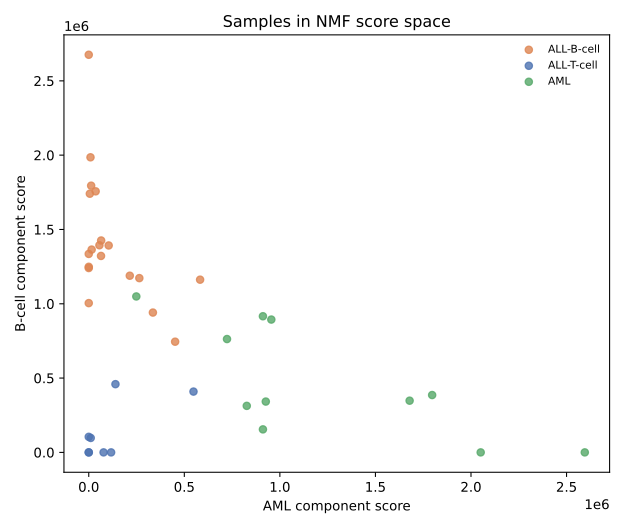
The score plot shows which samples carry the two displayed expression programs. AML samples generally extend along the AML axis and B-cell ALL samples along the B-cell axis. T-cell ALL samples lie closer to the origin because their strongest scores belong to the third, undisplayed component.
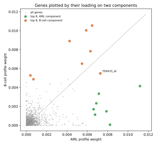
The loading plot explains what creates those sample directions. Genes near the AML axis contribute mainly to the AML profile, and genes near the B-cell axis contribute mainly to the B-cell profile. A gene far from both axes contributes to both profiles and therefore helps reconstruct both groups without separating them strongly.
Together, the plots connect the two sides of the factorization: W_named identifies the samples carrying each program, while H_named identifies the genes defining that program.