2  ICA with Python

Here we repeat that workflow in Python with scikit-learn. The simulation contains three latent signals, immune activation, metabolism, and cell cycle activity, that are mixed across genes. For the derivation of FastICA and the implementation from scratch, refer to the mathematics section in the previous chapter.

2.1 Setup

We use sklearn.decomposition.FastICA and sklearn.decomposition.PCA. Preprocessing is done with sklearn.preprocessing.StandardScaler, and plots are made with matplotlib.

NoteSoftware versions

numpy 2.5.3, pandas 3.0.6, scikit-learn 1.9.1, matplotlib 3.11.2. The whiten argument of FastICA changed its default in scikit-learn 1.3, so the exact argument names used below assume a reasonably recent scikit-learn version. Check sklearn.__version__ if anything below behaves differently.

2.2 Simulate expression data

The design matches the R example: 2,000 cells, 1,000 genes, and three latent sources. Immune activity has an exponential contribution, metabolism is normally distributed within each cluster, and cell cycle takes one of two values. A positive loading matrix mixes the sources across genes, after which Gaussian noise is added. The seed is fixed, but R and Python use different random-number generators, so the values are not expected to match across chapters.

Throughout this chapter, rows are cells and columns are genes.

import numpy as np
from sklearn.decomposition import PCA, FastICA
from sklearn.preprocessing import StandardScaler

rng = np.random.default_rng(123)

n_genes, n_cells, n_sources, n_clusters = 1000, 2000, 3, 5
cells_per_cluster = n_cells // n_clusters

cluster_means = np.array([
    [3.0, 0.5],   # Cluster 1: High immune, low metabolism
    [0.1, 2.0],   # Cluster 2: Low immune, high metabolism
    [1.5, 1.5],   # Cluster 3: Moderate all
    [3.0, 2.5],   # Cluster 4: High in all
    [0.1, 0.1],   # Cluster 5: Low in all
])

latent_blocks, cluster_labels = [], []
for i in range(n_clusters):
    immune = rng.exponential(1.0, cells_per_cluster) + cluster_means[i, 0]
    metabolism = rng.normal(cluster_means[i, 1], 0.5, cells_per_cluster)
    cell_cycle = rng.binomial(1, 0.5, cells_per_cluster) * 2 - 1
    latent_blocks.append(np.column_stack([immune, metabolism, cell_cycle]))
    cluster_labels += [f"Cluster {i + 1}"] * cells_per_cluster

latent_sources = np.vstack(latent_blocks)
cluster_labels = np.array(cluster_labels)

gene_loadings = np.abs(rng.standard_normal((n_genes, n_sources)))
expression_matrix = latent_sources @ gene_loadings.T
expression_matrix += rng.normal(scale=1.0, size=(n_cells, n_genes))

print("latent_sources:", latent_sources.shape)
print("expression_matrix:", expression_matrix.shape)

latent_sources: (2000, 3)
expression_matrix: (2000, 1000)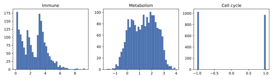

Figure 2.1: Distribution of the three simulated latent sources, before mixing. Immune activity is right-skewed, metabolism is approximately Gaussian, and cell cycle is a binary ±1 signal.

2.3 Use PCA as a reference

As a reference, we run PCA after centering and scaling each gene. StandardScaler uses the population standard deviation (ddof=0), whereas R’s scale() uses the sample standard deviation (ddof=1). In this example that difference multiplies every standardized gene by the same constant, so it does not change the PCA directions.

scaled_data = StandardScaler().fit_transform(expression_matrix)
pca = PCA(n_components=3)
pca_scores = pca.fit_transform(scaled_data)
print(pca_scores.shape)

(2000, 3)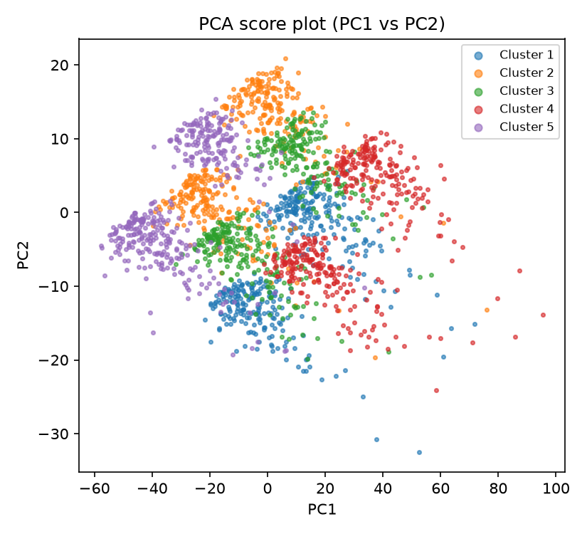

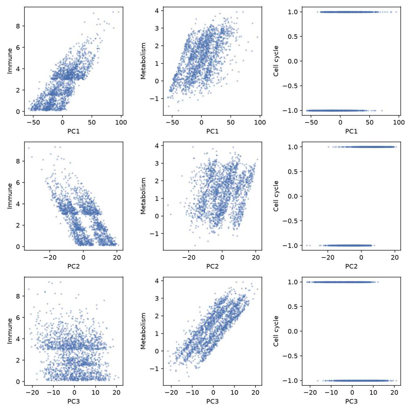
Figure 2.2: PCA score plot (PC1 vs PC2), colored by the five simulated biological clusters.

Figure 2.3: Each principal component plotted against each true latent source. Several relationships are strong, but each PC still combines more than one source rather than providing a one-to-one recovery.

PCA captures much of the simulated structure, but the panels show that a PC can be related to several sources. PCA orders directions by variance; it does not try to recover one independent process per component.

2.4 Fit FastICA

ica = FastICA(n_components=3, random_state=123, whiten="unit-variance")
S = ica.fit_transform(scaled_data)

print("S:", S.shape)
print("components_:", ica.components_.shape)
print("mixing_:", ica.mixing_.shape)
print("mean_:", ica.mean_.shape)
print("n_iter_:", ica.n_iter_)

S: (2000, 3)
components_: (3, 1000)
mixing_: (1000, 3)
mean_: (1000,)
n_iter_: 5

fit_transform(X) returns the estimated component scores S, with one row per cell and one column per component. This has the same layout as R’s ica_result$S.

• components_, shape (n_components, n_features): the unmixing operator. Applied to the centered data, it produces S. This plays the role of R’s W combined with the whitening step, not R’s A.
• mixing_, shape (n_features, n_components): the pseudo-inverse of components_, i.e. the matrix that maps sources back onto genes. This is the Python equivalent of R’s mixing matrix A, but transposed. R’s A is n.comp rows by p genes, so a component’s gene signature is a row of A. scikit-learn’s mixing_ is p genes by n_components, so a component’s gene signature is a column of mixing_.
• mean_, shape (n_features,): the per-gene mean subtracted before whitening. Only set when whiten is not False.

ImportantLocate component loadings in each implementation

In scikit-learn, components are columns of mixing_; in R’s fastICA, they are rows of A. Thus, mixing_[i, :] does not correspond to A[i, ].

2.5 Match components to the simulated sources

ICA components have no intrinsic order. To compare them with the known simulated signals, we calculate every component–source correlation and match on absolute correlation. Absolute values are used because an ICA component and all of its loadings may be multiplied by -1 without changing the fitted model.

import pandas as pd

corr = np.corrcoef(np.hstack([S, latent_sources]).T)[:3, 3:]
corr_df = pd.DataFrame(corr, index=["IC1", "IC2", "IC3"],
                        columns=["Immune", "Metabolism", "Cell cycle"])
print(corr_df.round(3))

best_match = np.abs(corr).argmax(axis=1)
names = ["Immune", "Metabolism", "Cell cycle"]
for i in range(3):
    j = best_match[i]
    print(f"IC{i+1} -> {names[j]} (r = {corr[i, j]:.3f})")

     Immune  Metabolism  Cell cycle
IC1  -0.028      -0.009      -0.999
IC2   0.028      -0.980      -0.004
IC3  -0.999      -0.193      -0.004
IC1 -> Cell cycle (r = -0.999)
IC2 -> Metabolism (r = -0.980)
IC3 -> Immune (r = -0.999)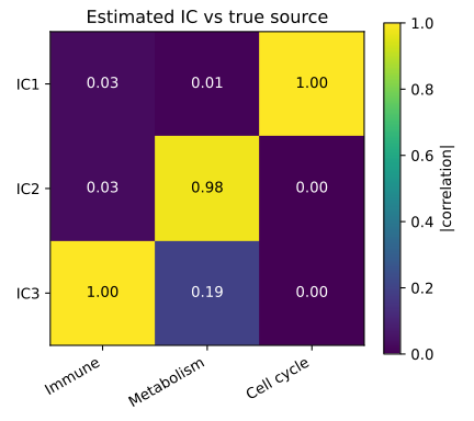

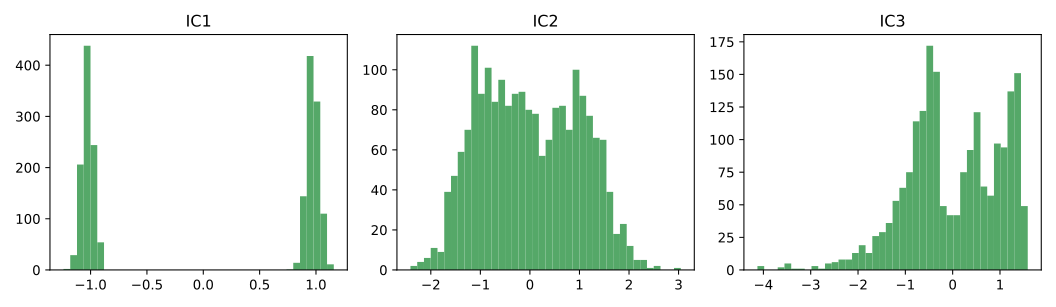
Figure 2.4: Absolute correlation between each estimated independent component and each true latent source. Each estimated component matches exactly one source closely, and the match is not in index order.

In this fit, IC1 matches cell cycle, IC2 matches metabolism, and IC3 matches immune activity. A different initialization may return the same signals in different columns or with reversed signs, so later analyses should match components by their values rather than by column number.

NoteComponent signs can reverse

All three correlations are negative in this fit. The magnitude of IC3’s correlation with immune activity (|r| = 0.999) indicates the quality of the match. Reversing both the IC3 scores and its column of mixing_ gives an equivalent representation of the fitted model.

2.6 Plot the component scores

import matplotlib.pyplot as plt

fig, ax = plt.subplots(figsize=(5.5, 5))
for k, label in enumerate(sorted(set(cluster_labels)), start=1):
    mask = cluster_labels == label
    ax.scatter(S[mask, 0], S[mask, 1], s=6, label=label, alpha=0.6)
ax.set_xlabel("IC1"); ax.set_ylabel("IC2"); ax.legend(markerscale=2, fontsize=8)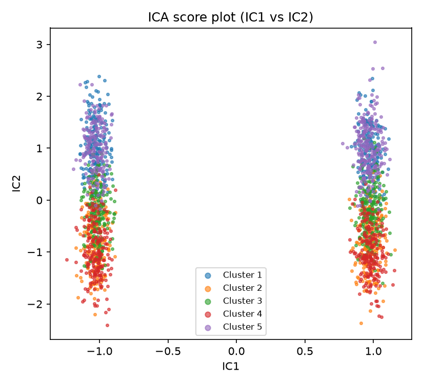

Figure 2.5: ICA score plot, IC1 vs IC2, colored by the simulated clusters. IC1 separates the two cell cycle states into vertical bands, while IC2 captures the metabolic signal and partially separates clusters with different metabolic means.

Figure 2.6: Distribution of each recovered independent component. Compare the shapes with the true source distributions in the first figure: IC1 is bimodal like cell cycle, IC2 is approximately bell-shaped like metabolism, and IC3 is left-skewed because it recovers the negative of immune activity.

2.7 Identify genes with large mixing weights

A component’s gene signature is a column of mixing_. For IC3, the component matched to immune activity above:

loadings = ica.mixing_[:, 2]
top_genes = np.argsort(-np.abs(loadings))[:10]
for g in top_genes:
    print(f"gene_{g + 1}: {loadings[g]:.3f}")

gene_801: -0.973
gene_443: -0.972
gene_497: -0.969
gene_745: -0.969
gene_16: -0.968
gene_85: -0.965
gene_535: -0.963
gene_462: -0.960
gene_407: -0.957
gene_800: -0.956

The largest absolute weights are negative because this fit represents immune activity with a reversed component sign. The signs are meaningful only relative to other genes in the same component; reversing all scores and weights would describe the same fit.

2.8 Useful FastICA arguments

Python (FastICA)	R (fastICA)	Notes
n_components	n.comp	Number of independent components to estimate.
algorithm (“parallel”, “deflation”)	alg.typ (“parallel”, “deflation”)	Whether components are extracted jointly (“parallel”) or one at a time (“deflation”).
fun (“logcosh”, “exp”, “cube”)	fun (“logcosh”, “exp”)	The contrast function approximating negentropy. scikit-learn additionally offers "cube", which R does not have.
fun_args (e.g. {"alpha": 1.0})	alpha	For fun="logcosh", R’s single alpha corresponds to fun_args={"alpha": ...} in Python.
max_iter	maxit	Maximum fixed-point iterations. Both default to 200.
tol	tol	Convergence tolerance. Both default to 1e-4.
random_state	(set via set.seed() before the call)	Controls the random initial unmixing matrix.
whiten (“unit-variance”, “arbitrary-variance”, False)	(whitening is always performed, via K)	scikit-learn can skip whitening if the data is already whitened. R’s fastICA always whitens internally.

Notewhiten default changed in scikit-learn 1.3

Before scikit-learn 1.3, whiten defaulted to True and used what is now called "arbitrary-variance" scaling. From 1.3 onward the default is "unit-variance", which rescales each recovered source to unit variance. Check sklearn.__version__ before relying on this default in other environments.

2.9 Whitening

FastICA whitens the data internally before its fixed-point iterations. The whitening derivation in the previous chapter explains this step and shows its manual implementation.

The next chapter applies ICA in both R and Python to a real gene expression dataset.